
Patient Characteristics and Readmission Modeling
Patient Characteristics and Readmission Modeling
1. Background
1.1. Introduction
A healthcare organization has engaged our team to conduct a comprehensive analysis of ten years of patient readmission data following discharge. The objective is to evaluate whether factors such as initial diagnoses, number of procedures, and other clinical variables can improve the prediction of readmission likelihood. The insights from this analysis will support more proactive patient care strategies, enabling targeted follow-up and resource allocation for individuals at higher risk of readmission.
1.2. Objectives
The main objective of this report is to explore patient characteristics and readmissions. It specifically aims to:
- Describe the overall and by age characteristics of the patients.
- Investigate and model the patient readmissions by their representing features.
- Identify patient groups with the best readmission rates.
1.3. Libraries & Functions
# Load required packages
library(tidyverse)
library(dplyr)
library(ggplot2)
library(Amelia)
library(summarytools)
library(scales)
library(ggchicklet)
library(ggthemes)
library(ggpubr)
library(rwantshue)
library(questionr)

# ========================================================
# Function: GroupedMedian()
# Purpose: Compute the median of grouped data
# Reference: Mahto (2013)
# ========================================================

GroupedMedian <- function(frequencies, intervals, sep = NULL, trim = NULL) {

  # ----------------------------------------------------------
  # Step 1. Preprocessing intervals
  # ----------------------------------------------------------
  # If "sep" is specified, attempt to parse textual intervals
  # into numeric lower and upper boundaries.
  # Example: "20-29" → c(20, 29)
  if (!is.null(sep)) {
    if (is.null(trim)) pattern <- ""
    else if (trim == "cut") pattern <- "\\[|\\]|\\(|\\)"
    else pattern <- trim

    # Clean intervals and split into numeric matrix
    intervals <- sapply(
      strsplit(gsub(pattern, "", intervals), sep),
      as.numeric
    )
  }

  # ----------------------------------------------------------
  # Step 2. Calculate midpoints and cumulative frequencies
  # ----------------------------------------------------------
  Midpoints <- rowMeans(intervals)
  cf <- cumsum(frequencies)

  # ----------------------------------------------------------
  # Step 3. Identify the median class
  # ----------------------------------------------------------
  Midrow <- findInterval(max(cf) / 2, cf) + 1

  # ----------------------------------------------------------
  # Step 4. Extract parameters for grouped median formula
  # ----------------------------------------------------------
  L   <- intervals[1, Midrow]       # Lower class boundary of median class
  h   <- diff(intervals[, Midrow])  # Width of the median class
  f   <- frequencies[Midrow]        # Frequency of median class
  cf2 <- cf[Midrow - 1]             # Cumulative frequency before median class
  n_2 <- max(cf) / 2                # Half of total frequency (n/2)

  # ----------------------------------------------------------
  # Step 5. Apply the grouped median formula
  # ----------------------------------------------------------
  # Median = L + ((n/2 – cf_before) / f_median) * class_width
  median_value <- L + (n_2 - cf2) / f * h

  # Return median
  unname(median_value)
}

# ======================================================
# Function: plot_distribution()
# Purpose: Create standardized histogram + density plots
# ======================================================

plot_distribution <- function(data, var,
                              fig_title, x_label,
                              binwidth = 1,
                              x_breaks = NULL, y_breaks = NULL,
                              x_limits = NULL, y_limits = NULL,
                              mean_x_offset = 0, mean_y = NULL,
                              fill_color = "#5AA7A7", density_color = "#FF6666",
                              mean_color = "red") {

  # Evaluate the variable input
  var <- rlang::enquo(var)

  # Compute variable mean
  var_mean <- mean(dplyr::pull(data, !!var), na.rm = TRUE)

  # Build the plot
  p <- ggplot(data, aes(x = !!var)) +
    geom_histogram(aes(y = after_stat(density)),
                   colour = "white",
                   fill = fill_color,
                   binwidth = binwidth) +
    geom_density(alpha = 0.2, fill = density_color) +
    geom_vline(aes(xintercept = var_mean),
               col = mean_color,
               linewidth = 0.6) +
    ggtitle(fig_title) +
    labs(x = x_label, y = "Density\n") +
    scale_x_continuous(expand = c(0.01, 0),
                       breaks = x_breaks,
                       limits = x_limits) +
    scale_y_continuous(expand = c(0.01, 0),
                       breaks = y_breaks,
                       limits = y_limits) +
    theme_economist() +
    scale_color_economist() +
    theme(
      plot.title = element_text(size = 12),
      panel.grid.minor = element_line(color = "grey",
                                      linetype = "dashed",
                                      linewidth = 0.3),
      panel.grid.major = element_line(color = "grey",
                                      linetype = "dashed",
                                      linewidth = 0.3)
    ) +
    annotate("text",
             x = var_mean + mean_x_offset,
             y = mean_y,
             label = paste("Mean =", round(var_mean, 4)),
             color = mean_color,
             size = 3.5)

  return(p)
}
1.4. Dataset
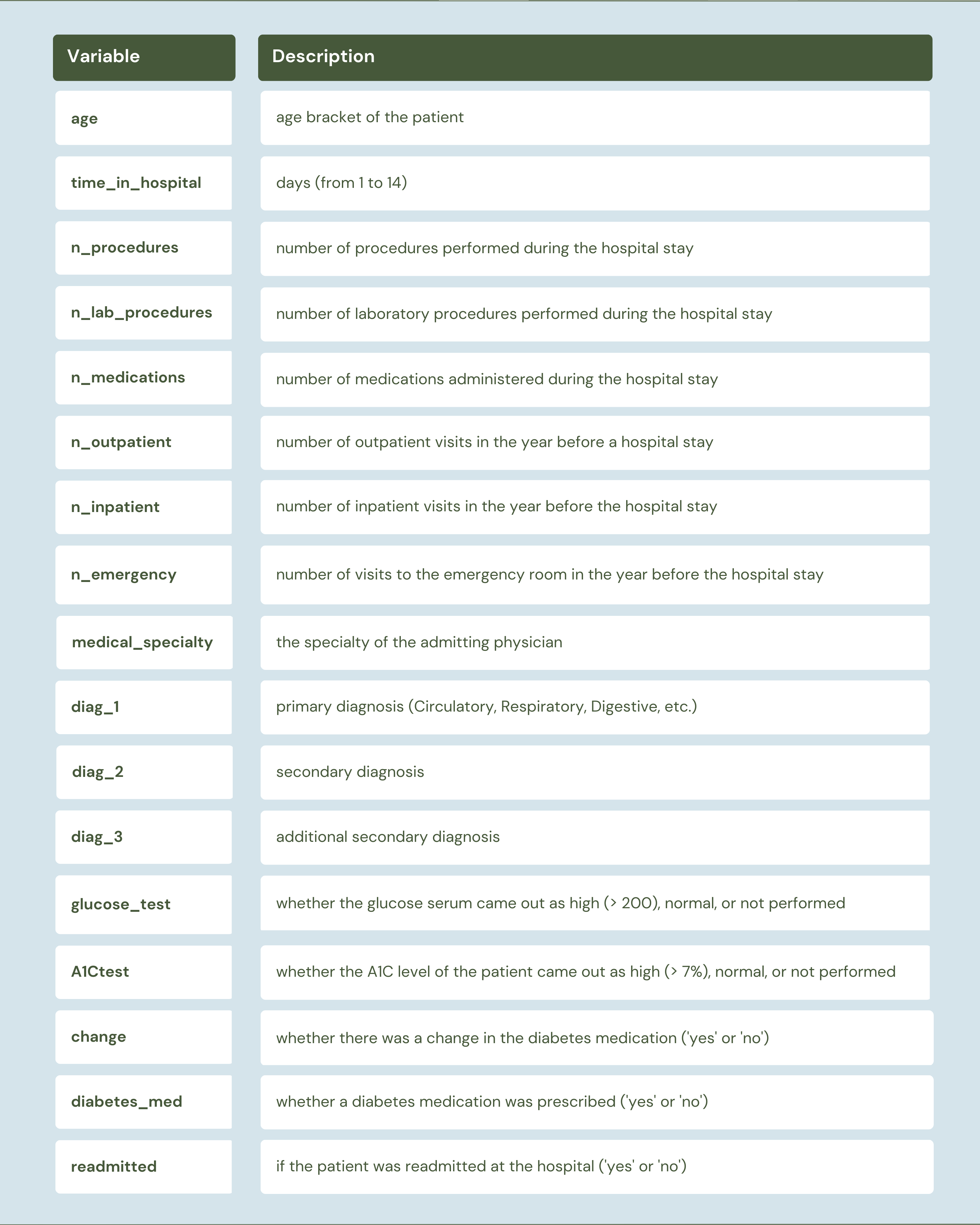
The dataset referenced was part of the clinical care system at 130 hospitals and integrated delivery networks in the United States (Strack et al., 2014).
# Read 'readmissions' dataset
readmissions <- read_csv('data/hospital_readmissions.csv', show_col_types = FALSE)
#glimpse(readmissions)

# Mutate 'Missing' values to NA & convert character variables to factors
readmissions <- readmissions %>%
    mutate_all(~ if_else(.x == "Missing", NA, .x)) %>%
    mutate_if(is.character, as.factor)
head(readmissions)
| age <fct> | time_in_hospital <dbl> | n_lab_procedures <dbl> | n_procedures <dbl> | n_medications <dbl> | n_outpatient <dbl> | n_inpatient <dbl> | n_emergency <dbl> | medical_specialty <fct> | diag_1 <fct> | diag_2 <fct> | diag_3 <fct> | glucose_test <fct> | A1Ctest <fct> | change <fct> | diabetes_med <fct> | readmitted <fct> |
|---|---|---|---|---|---|---|---|---|---|---|---|---|---|---|---|---|
| [70-80) | 8 | 72 | 1 | 18 | 2 | 0 | 0 | NA | Circulatory | Respiratory | Other | no | no | no | yes | no |
| [70-80) | 3 | 34 | 2 | 13 | 0 | 0 | 0 | Other | Other | Other | Other | no | no | no | yes | no |
| [50-60) | 5 | 45 | 0 | 18 | 0 | 0 | 0 | NA | Circulatory | Circulatory | Circulatory | no | no | yes | yes | yes |
| [70-80) | 2 | 36 | 0 | 12 | 1 | 0 | 0 | NA | Circulatory | Other | Diabetes | no | no | yes | yes | yes |
| [60-70) | 1 | 42 | 0 | 7 | 0 | 0 | 0 | InternalMedicine | Other | Circulatory | Respiratory | no | no | no | yes | no |
| [40-50) | 2 | 51 | 0 | 10 | 0 | 0 | 0 | NA | Other | Other | Other | no | no | no | no | yes |
# Check NA's
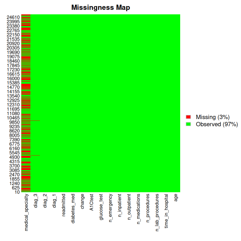
colSums(is.na(readmissions)) # NA's per column
which(colSums(is.na(readmissions))>0) # column indices containing NA's
missmap(readmissions, col=c("red", "green"), legend=FALSE) # missingness map
          age  time_in_hospital  n_lab_procedures      n_procedures
            0                 0                 0                 0
n_medications      n_outpatient       n_inpatient       n_emergency
            0                 0                 0                 0
medical_specialty            diag_1            diag_2            diag_3
            12382                 4                42               196
 glucose_test           A1Ctest            change      diabetes_med
            0                 0                 0                 0
   readmitted
            0


medical_specialty            diag_1            diag_2            diag_3
                9                10                11                12
2. Results & Discussion
2.1. Descriptive Statistics
The following information describe the characteristics of the sample composing of 25,000 patients admitted to the hospital after being discharged.
2.1.1. Numerical
2.1.1.2. Time in Hospital
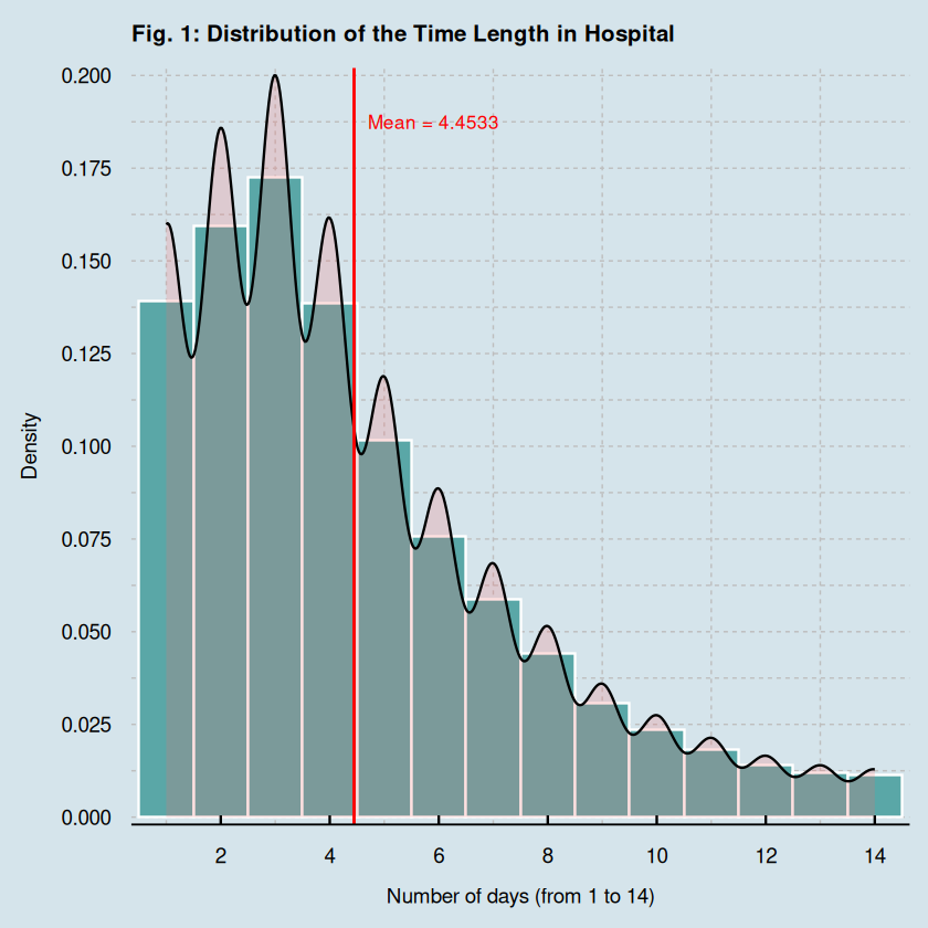
The mean and median lengths of hospital stay are 4.45 and 4 days, respectively, with a standard deviation of approximately 3 days. As shown in Figure 2, the distribution of hospital stay duration is positively skewed, indicating that most patients were hospitalized for shorter periods.
| Variable | N | Mean | Std.Dev | Min | Q1 | Median | Q3 | Max |
|---|---|---|---|---|---|---|---|---|
| time_in_hospital | 25,000 | 4.4533 | 3.0015 | 1 | 2 | 4 | 6 | 14 |
# Summary statistics for numerical variables
sum_stats <- descr(readmissions) %>%
  t() %>%
  as.data.frame() %>%
  tibble::rownames_to_column("Variable") %>%
  select(Variable, N, Mean, Std.Dev, Min, Q1, Median, Q3, Max) %>%
  mutate(across(where(is.numeric), ~ round(.x, 4)))

## Time in Hospital

# Fig. 1
plot_distribution(readmissions, time_in_hospital,
  fig_title = "Fig. 1: Distribution of the Time Length in Hospital\n",
  x_label = "\nNumber of days (from 1 to 14)",
  binwidth = 1,
  x_breaks = seq(0, 14, 2),
  y_breaks = seq(0, 0.20, 0.025),
  mean_x_offset = 1.45,
  mean_y = 0.1875
)

# Summary statistics
sum_stats %>% filter(Variable == "time_in_hospital")
2.1.1.3. Number of Procedures
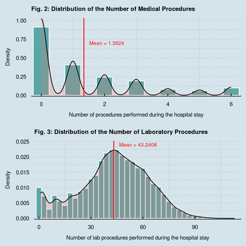
During hospitalization, patients underwent an average of approximately one medical procedure and 43 to 44 laboratory procedures, with standard deviations of 1.72 and 19.82, respectively. Figures 3 and 4 further illustrate distinct distributional patterns between the two procedure types: medical procedures exhibit positive skewness, indicating that most patients underwent few procedures, whereas laboratory procedures display a nearly symmetric distribution, suggesting a more consistent level of administration across patients.
| Variable | N | Mean | Std.Dev | Min | Q1 | Median | Q3 | Max |
|---|---|---|---|---|---|---|---|---|
| n_procedures | 25,000 | 1.3524 | 1.7152 | 0 | 0 | 1 | 2 | 6 |
| n_lab_procedures | 25,000 | 43.2408 | 19.8186 | 1 | 31 | 44 | 57 | 113 |
# Fig. 2: Number of Procedures
n_procedures_hs_dst_plot <- plot_distribution(readmissions, n_procedures,
  fig_title = "Fig. 2: Distribution of the Number of Medical Procedures\n",
  x_label = "\nNumber of procedures performed during the hospital stay",
  binwidth = 0.5,
  x_breaks = seq(0, 7, 2),
  y_breaks = seq(0, 1, 0.25),
  mean_x_offset = 0.72,
  mean_y = 0.7
)

# Fig. 3: Number of Lab Procedures
n_lab_procedures_hs_dst_plot <- plot_distribution(readmissions, n_lab_procedures,
  fig_title = "Fig. 3: Distribution of the Number of Laboratory Procedures\n",
  x_label = "\nNumber of lab procedures performed during the hospital stay",
  binwidth = 3,
  x_breaks = seq(0, 120, 30),
  y_breaks = seq(0, 0.025, 0.005),
  y_limits = c(0, 0.025),
  mean_x_offset = 14,
  mean_y = 0.024
)

ggarrange(n_procedures_hs_dst_plot, n_lab_procedures_hs_dst_plot, ncol = 1, nrow = 2)

# Summary statistics
sum_stats %>% filter(str_detect(Variable, "procedures"))
2.1.1.4. Number of Medications
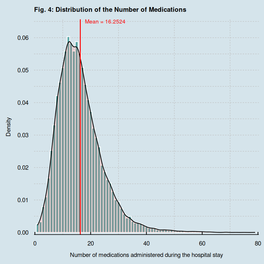
The average number of medications administered during hospitalization is 16.25, with a median of 15 and a standard deviation of 8.06. This indicates that medication usage varied notably among patients, with some receiving substantially more medications than others. The distribution is slightly right-skewed, suggesting that while most patients received a moderate number of medications, a smaller proportion were prescribed a relatively higher number.
| Variable | N | Mean | Std.Dev | Min | Q1 | Median | Q3 | Max |
|---|---|---|---|---|---|---|---|---|
| n_medications | 25,000 | 16.2524 | 8.0605 | 1 | 11 | 15 | 20 | 79 |
# Fig. 4: Number of Medications
plot_distribution(readmissions, n_medications,
  fig_title = "Fig. 4: Distribution of the Number of Medications\n",
  x_label = "\nNumber of medications administered during the hospital stay",
  binwidth = 1,
  x_breaks = seq(0, 80, 20),
  y_breaks = seq(0, 0.065, 0.01),
  y_limits = c(0, 0.065),
  mean_x_offset = 9,
  mean_y = 0.065
)

# Summary statistics
sum_stats %>% filter(Variable == "n_medications")
2.1.1.5. Number of Visits
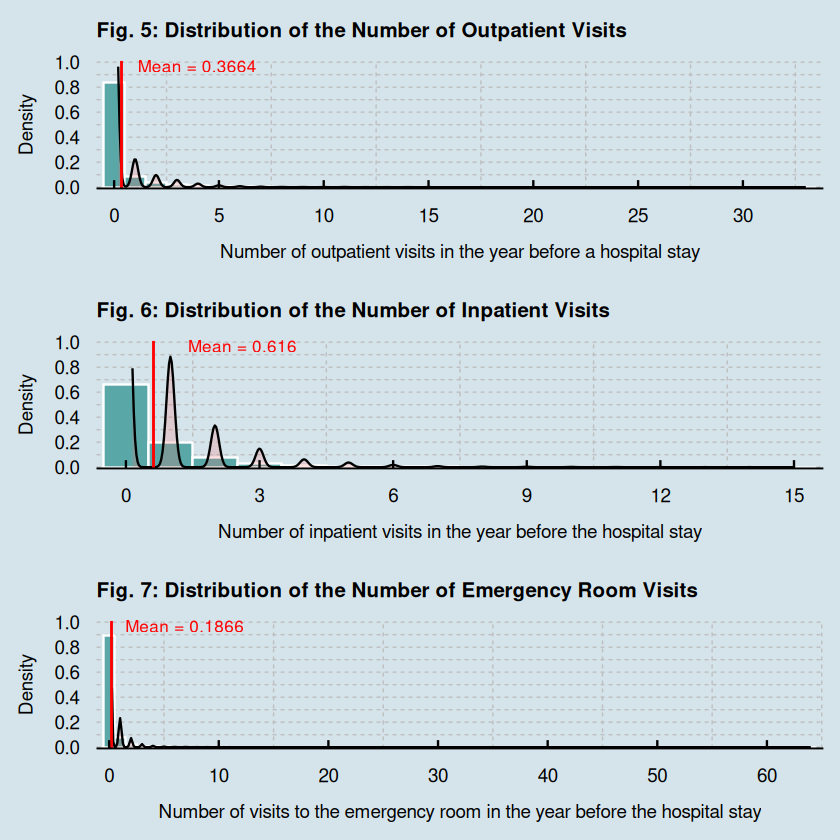
The average numbers of outpatient, inpatient, and emergency room visits in the year preceding hospitalization are all below one, with median values of zero across visit types. This indicates that most patients had no recorded visits prior to admission. The moderate standard deviations suggest some variation in visit frequency, as a small subset of patients had multiple visits. Overall, the positively skewed distributions imply that frequent pre-hospital visits were uncommon within the patient population.
| Variable | N | Mean | Std.Dev | Min | Q1 | Median | Q3 | Max |
|---|---|---|---|---|---|---|---|---|
| n_outpatient | 25,000 | 0.3664 | 1.1955 | 0 | 0 | 0 | 0 | 33 |
| n_inpatient | 25,000 | 0.6160 | 1.1780 | 0 | 0 | 0 | 1 | 15 |
| n_emergency | 25,000 | 0.1866 | 0.8859 | 0 | 0 | 0 | 0 | 64 |
# Fig. 5: Outpatient Visits
n_outpatient_hs_dst_plot <- plot_distribution(readmissions, n_outpatient,
  fig_title = "Fig. 5: Distribution of the Number of Outpatient Visits\n",
  x_label = "\nNumber of outpatient visits in the year before a hospital stay",
  binwidth = 1,
  x_breaks = seq(0, 35, 5),
  y_breaks = seq(0, 1, 0.2),
  y_limits = c(0, 1),
  mean_x_offset = 3.6,
  mean_y = 0.97
)

# Fig. 6: Inpatient Visits
n_inpatient_hs_dst_plot <- plot_distribution(readmissions, n_inpatient,
  fig_title = "Fig. 6: Distribution of the Number of Inpatient Visits\n",
  x_label = "\nNumber of inpatient visits in the year before the hospital stay",
  binwidth = 1,
  x_breaks = seq(0, 18, 3),
  y_breaks = seq(0, 1, 0.2),
  y_limits = c(0, 1),
  mean_x_offset = 2,
  mean_y = 0.97
)

# Fig. 7: Emergency Room Visits
n_emergency_hs_dst_plot <- plot_distribution(readmissions, n_emergency,
  fig_title = "Fig. 7: Distribution of the Number of Emergency Room Visits\n",
  x_label = "\nNumber of visits to the emergency room in the year before the hospital stay",
  binwidth = 1,
  x_breaks = seq(0, 65, 10),
  y_breaks = seq(0, 1, 0.2),
  y_limits = c(0, 1),
  mean_x_offset = 6.7,
  mean_y = 0.97
)

ggarrange(n_outpatient_hs_dst_plot, n_inpatient_hs_dst_plot, n_emergency_hs_dst_plot, ncol = 1, nrow = 3)

# Summary statistics
sum_stats %>% filter(Variable %in% c("n_outpatient", "n_inpatient", "n_emergency"))
2.1.2. Categorical
2.1.2.1. Age
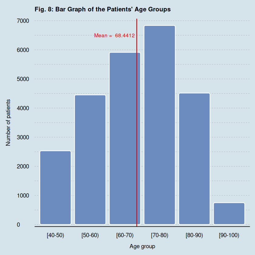
With a grouped mean of 68.4 years and a median of 69.3 years, the age distribution appears fairly symmetric and moderately dispersed (SD = 13.2). As seen in Figure 8, most patients admitted were between 50 and 90 years old.
| Age Group | Frequency | Cumulative Frequency | Cumulative Relative Frequency |
|---|---|---|---|
| [40–50) | 2,532 | 2,532 | 0.1013 |
| [50–60) | 4,452 | 6,984 | 0.2794 |
| [60–70) | 5,913 | 12,897 | 0.5159 |
| [70–80) | 6,837 | 19,734 | 0.7894 |
| [80–90) | 4,516 | 24,250 | 0.9700 |
| [90–100) | 750 | 25,000 | 1.0000 |
| Variable | Mean | Std.Dev | Median |
|---|---|---|---|
| Age group | 68.4412 | 13.1561 | 69.3286 |
## Age

# Frequency table
age_fdt <- readmissions %>%
  count(age, name = "n") %>%
  mutate(
    lower = as.numeric(str_extract(age, "(?<=\\[|\\()(\\d+)")),
    upper = as.numeric(str_extract(age, "(\\d+)(?=\\)|\\])")),
    class_interval = paste(lower, upper, sep = "-"),
    class_mark = (lower + upper) / 2,
    cf = cumsum(n),
    crf = cf/sum(n),
    n_times_cm = n * class_mark
  ) %>%
  select(age, class_interval, everything())

# Fig. 8
age_bar_plot <- ggplot(age_fdt, aes(group=1)) +
	geom_chicklet(aes(x = age,
                      y = n,
					  group=1),
                  color="white",
                  fill="#6C8CBF",
                  radius = grid::unit(1, "mm"), position="stack") +

	# Plot mean line
	geom_vline(xintercept=3.344, color="red", linewidth=0.6) +

	ggtitle("Fig. 8: Bar Graph of the Patients' Age Groups\n") +
	labs(x="\nAge group", y="Number of patients\n") +
	scale_y_continuous(expand = c(0.01, 0), limits = c(0,7000),
                      breaks = seq(0, 7000, by=1000)) +
	theme_economist() +
	scale_color_economist() +
	theme(plot.title = element_text(size= 12),
          panel.grid.minor = element_line(color="grey",
                                          linetype="dashed",
                                          linewidth=0.3),
		  panel.grid.major = element_line(color="grey",
                                          linetype="dashed",
                                          linewidth=0.3),
          axis.ticks = element_blank()
         ) +
	annotate("text", x=2.7, y=6500,
			 label=paste("Mean = ",sum(age_fdt$n_times_cm)/sum(age_fdt$n)),
			 color="red",
			 size=3.5)

# Summary statistics
age_stats <- age_fdt %>%
  summarise(
    Variable = "Age group",
    Mean = sum(n * class_mark) / sum(n),
    Std.Dev = sqrt(sum(n * (class_mark - (sum(n * class_mark) / sum(n)))^2) / sum(n)),
    Median = GroupedMedian(frequencies = n, intervals = class_interval, sep = "-")
  ) %>%
  mutate(across(where(is.numeric), ~ round(.x, 4)))
2.1.2.1. Medical Specialty
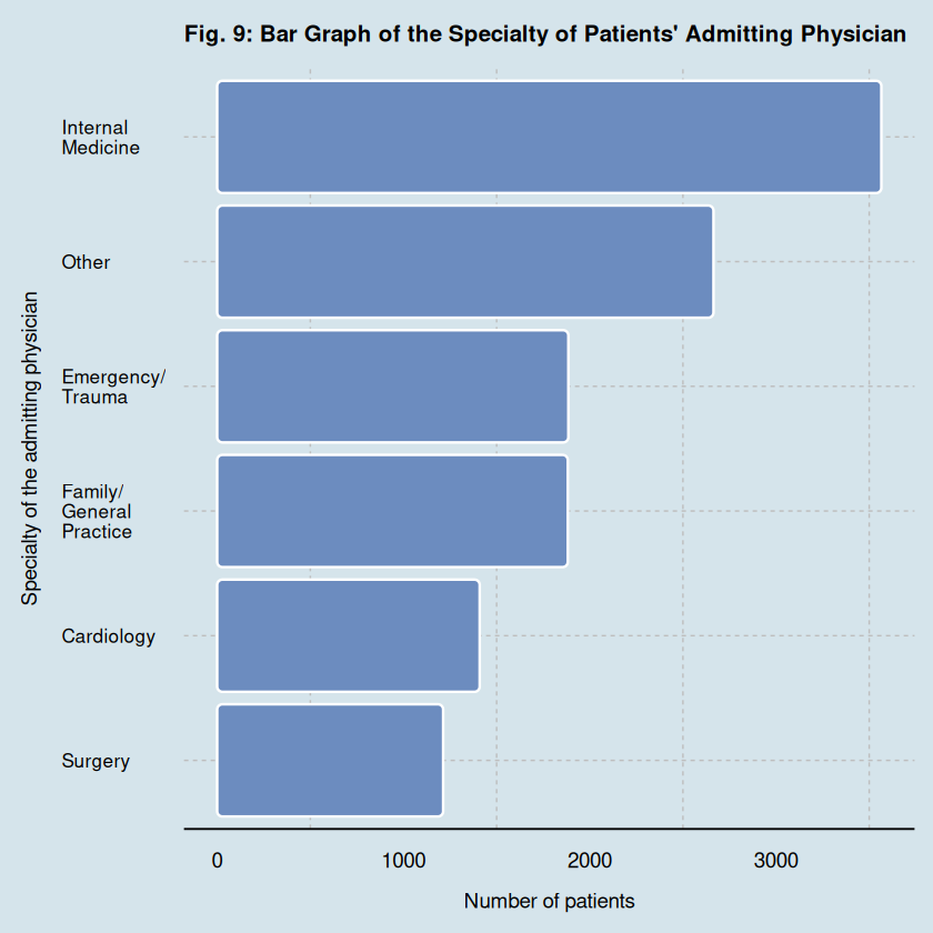
Out of the 12,618 patients with a recorded admitting physician, Internal Medicine was the most common specialty, accounting for 3,565 patients (28.25%). This was followed by physicians classified under Other specialties (21.11%), Emergency/Trauma (14.94%), and Family/General Practice (14.92%). Fewer patients were admitted by specialists in Cardiology (11.17%) and Surgery (9.61%).
| Medical Specialty | Frequency | Percentage |
|---|---|---|
| Internal Medicine | 3565 | 28.25% |
| Other | 2664 | 21.11% |
| Emergency/Trauma | 1885 | 14.94% |
| Family/GeneralPractice | 1882 | 14.92% |
| Cardiology | 1409 | 11.17% |
| Surgery | 1213 | 9.61% |
# Frequency table
medical_specialty_fdt <- readmissions %>%
	select(medical_specialty) %>%
  filter(!is.na(medical_specialty)) %>%
	group_by(medical_specialty) %>%
	count() %>%
	ungroup() %>%
	mutate(perc = label_percent(accuracy=0.01)(n/sum(n))) %>%
	arrange(desc(n))

# Fig. 9
medical_specialty_bar_plot <- ggplot(medical_specialty_fdt %>%
                    filter(!is.na(medical_specialty))) +
  geom_chicklet(aes(x = fct_reorder(medical_specialty,n),
                      y = n),
                  fill=c("#6C8CBF"),
                  color="white",
                  radius = grid::unit(1, "mm"), position="stack",
          na.rm = TRUE) +
  coord_flip() +
  ggtitle("Fig. 9: Bar Graph of the Specialty of Patients' Admitting Physician \n") +
  labs(y="\nNumber of patients", x="Specialty of the admitting physician\n") +
  theme_economist() +
  scale_color_economist() +
  theme(legend.position="bottom",
          legend.text = element_text(margin = margin(r = 2, unit = "pt"),
                                     size = 10),
          axis.ticks = element_blank(),
      axis.text.y = element_text(size=10),
          legend.title = element_text(face="bold",
                                      size = 12),
          panel.grid.minor = element_line(color="grey",
                                          linetype="dashed",
                                          linewidth=0.3),
      panel.grid.major = element_line(color="grey",
                                          linetype="dashed",
                                          linewidth=0.3),
          plot.title = element_text(hjust = 0,
                                    size= 12),
          legend.box.margin = margin(t=0, b=0, l=-95, unit='pt'))  +
  scale_x_discrete(expand = c(0.11, 0),
           labels = rev(c("Internal\nMedicine",
                "Other",
                "Emergency/\nTrauma",
                "Family/\nGeneral\nPractice",
                  "Cardiology",
                  "Surgery"))
           )
2.1.2.2. Diagnoses
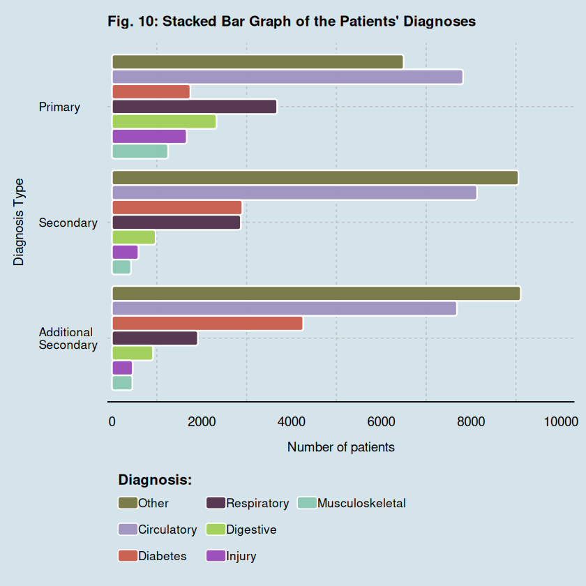
Across all diagnosis types, circulatory diseases were the most frequently reported, accounting for approximately 31% to 33% for each. Among primary diagnoses, circulatory conditions were followed by respiratory diseases (14.72%). For secondary diagnoses, diabetes (11.64%) and respiratory diseases (11.51%) occurred with nearly equal frequency, whereas among additional secondary diagnoses, diabetes (17.18%) ranked as the second most common.
Furthermore, the distribution of digestive, injury, and musculoskeletal diagnoses was relatively consistent between secondary and additional secondary types, suggesting a similar pattern of occurrence for these less frequent diagnoses.
| Diagnosis Type | Diagnosis | Frequency | Percentage |
|---|---|---|---|
| Primary | Circulatory | 7,824 | 31.30% |
| Primary | Respiratory | 3,680 | 14.72% |
| Primary | Digestive | 2,329 | 9.32% |
| Primary | Diabetes | 1,747 | 6.99% |
| Primary | Injury | 1,666 | 6.67% |
| Primary | Musculoskeletal | 1,252 | 5.01% |
| Primary | Other | 6,498 | 26.00% |
| Secondary | Circulatory | 8,134 | 32.59% |
| Secondary | Diabetes | 2,906 | 11.64% |
| Secondary | Respiratory | 2,872 | 11.51% |
| Secondary | Digestive | 973 | 3.90% |
| Secondary | Injury | 591 | 2.37% |
| Secondary | Musculoskeletal | 426 | 1.71% |
| Secondary | Other | 9,056 | 36.28% |
| Additional Secondary | Circulatory | 7,686 | 30.99% |
| Additional Secondary | Diabetes | 4,261 | 17.18% |
| Additional Secondary | Respiratory | 1,915 | 7.72% |
| Additional Secondary | Digestive | 916 | 3.69% |
| Additional Secondary | Injury | 464 | 1.87% |
| Additional Secondary | Musculoskeletal | 455 | 1.83% |
| Additional Secondary | Other | 9,107 | 36.72% |
# Frequency table
diag_tbl <- readmissions %>%
  select(diag_1, diag_2, diag_3) %>%
  pivot_longer(
    cols = everything(),
    names_to = "diag_type",
    values_to = "diag"
  ) %>%
  filter(!is.na(diag)) %>%
  group_by(diag_type, diag) %>%
  summarize(n = n(), .groups = "drop_last") %>%
  mutate(perc = n / sum(n)) %>%
  ungroup() %>%
  arrange(diag_type, desc(n)) %>%
  mutate(perc = label_percent(accuracy = 0.01)(perc))

# Colorize the Physician's Specialty
color_scheme1 <- iwanthue(seed=1234, force_init=TRUE)
diag_colors <- color_scheme1$hex(length(levels(factor(diag_tbl$diag))))

# Convert diagnostic type to factor and specify level order
diag_tbl$diag_type <- factor(diag_tbl$diag_type, levels=c('diag_3', 'diag_2', 'diag_1'))

# Fig. 10
diag_stacked_bar_plot <- ggplot(diag_tbl %>% filter(!is.na(diag))) +
  geom_chicklet(aes(x = diag_type, y = n,
                      fill = fct_reorder(diag, n)),
                  color="white",
                  alpha=0.95,
                  radius = grid::unit(0.75, "mm"),
                  position="dodge") +
  coord_flip() +
  ggtitle("Fig. 10: Stacked Bar Graph of the Patients' Diagnoses\n") +
  labs(x="Diagnosis Type\n", y="\nNumber of patients", fill="Diagnosis: ") +
  theme_economist() +
  scale_color_economist() +
    guides(fill = guide_legend(ncol=3,
                               reverse = TRUE,
                               override.aes = list(shape = 15,
                                                   size = 4),
                               title.position="top")) +
  theme(legend.position="bottom",
          legend.text = element_text(margin = margin(r = 2, unit = "pt"),
                                     size = 10),
          axis.ticks = element_blank(),
      axis.text.y = element_text(size=10),
          legend.title = element_text(face="bold",
                                      size = 12),
          panel.grid.minor = element_line(color="grey",
                                          linetype="dashed",
                                          linewidth=0.3),
      panel.grid.major = element_line(color="grey",
                                          linetype="dashed",
                                          linewidth=0.3),
          plot.title = element_text(hjust = 0,
                                    size= 12),
          legend.box.margin = margin(t=0, b=0, l=-135, unit='pt')) +
  scale_fill_manual(values = diag_colors,
           ) +
  scale_y_continuous(expand = c(0.01, 0),
                   limits = c(0, 10200),
                       breaks = seq(0, 10200, by=2000)) +
  scale_x_discrete(expand = c(0.275, 0),
                    labels = c("Additional\nSecondary", "Secondary", "Primary"))
2.1.2.3. Prediabetes Test
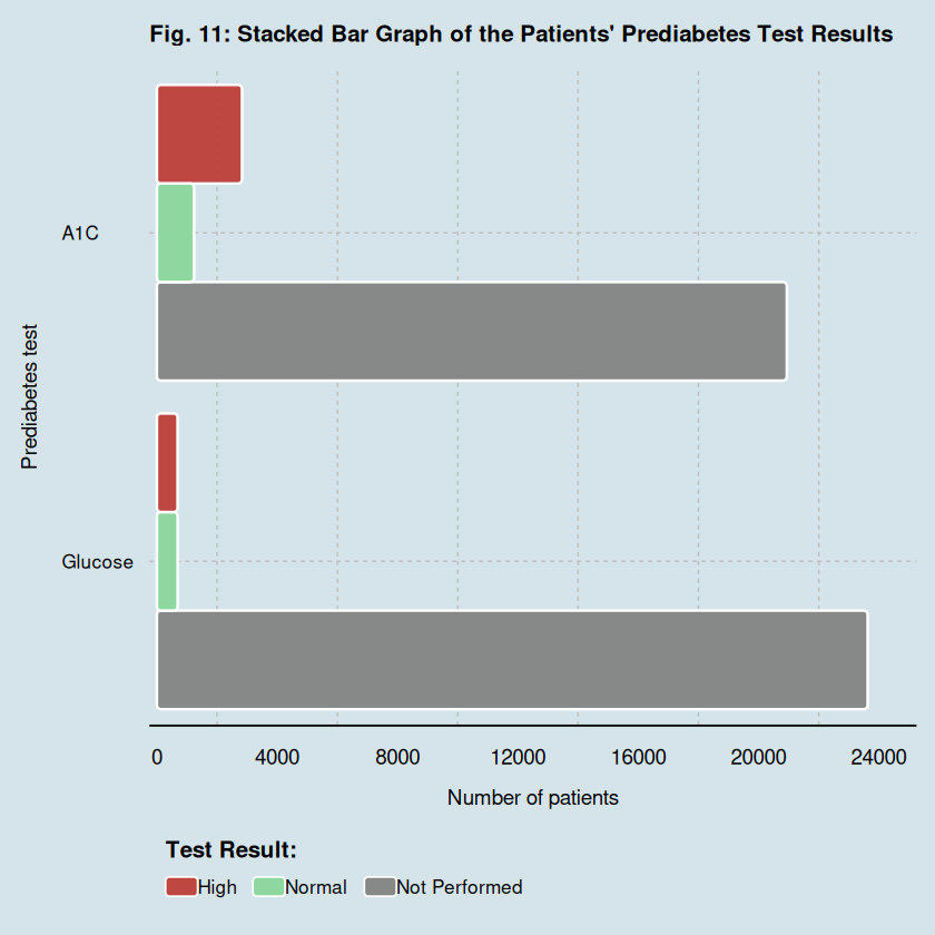
A total of 20,938 (83.75%) had not performed an A1C test, while 23,625 (94.50%) had not performed a glucose test. For those who had performed, however, a high result was seen more than a normal one for A1C tests and almost equal number in high and normal results for glucose test.
| Prediabetes Test | Result | Frequency | Percentage |
|---|---|---|---|
| A1C | Not Performed | 20,938 | 83.75% |
| A1C | High | 2,827 | 11.31% |
| A1C | Normal | 1,235 | 4.94% |
| Glucose | Not Performed | 23,625 | 94.50% |
| Glucose | Normal | 689 | 2.76% |
| Glucose | High | 686 | 2.74% |
# Frequency table
diab_test_tbl <- readmissions %>%
  select(glucose_test, A1Ctest) %>%
  rename(
    Glucose = glucose_test,
    A1C = A1Ctest
  ) %>%
  pivot_longer(
    cols = everything(),
    names_to = "prediab_test",
    values_to = "result"
  ) %>%
  filter(!is.na(result)) %>%
  group_by(prediab_test, result) %>%
  summarize(n = n(), .groups = "drop_last") %>%
  mutate(perc = n / sum(n)) %>%
  ungroup() %>%
  arrange(prediab_test, desc(n)) %>%
  mutate(perc = label_percent(accuracy = 0.01)(perc))

# Convert test result type to factor and specify level order
diab_test_tbl$result <- factor(diab_test_tbl$result, levels=c("no",'normal','high'))

# Fig. 11
diab_test_stacked_bar_plot <- ggplot(diab_test_tbl) +
  geom_chicklet(aes(x = fct_reorder(prediab_test, n), y = n,
                      fill = result),
                  color="white",
                  alpha=0.95,
                  radius = grid::unit(0.75, "mm"),
                  position="dodge") +
  coord_flip() +
  scale_fill_manual(values = c("#838484", "#8BD69D", "#BD3E38"),
                      labels = c("Not Performed", "Normal", "High")
                     ) +
  ggtitle("Fig. 11: Stacked Bar Graph of the Patients' Prediabetes Test Results\n") +
  labs(x="Prediabetes test\n", y="\nNumber of patients", fill="Test Result:  ") +
  theme_economist() +
  scale_color_economist() +
    guides(fill = guide_legend(ncol=3,
                               reverse = TRUE,
                               override.aes = list(shape = 15,
                                                   size = 4),
                               title.position="top")) +
  theme(legend.position="bottom",
          legend.text = element_text(margin = margin(r = 2, unit = "pt"),
                                     size = 10),
          legend.title = element_text(face="bold",
                                      size = 12),
          axis.ticks = element_blank(),
      axis.text.y = element_text(size=10),
          panel.grid.minor = element_line(color="grey",
                                          linetype="dashed",
                                          linewidth=0.3),
      panel.grid.major = element_line(color="grey",
                                          linetype="dashed",
                                          linewidth=0.3),
          plot.title = element_text(hjust = 0,
                                    size= 12),
          legend.box.margin = margin(t=0, b=0, l=-200, unit='pt')) +
  scale_y_continuous(expand = c(0.01, 0),
                   limits = c(0, 25000),
                       breaks = seq(0, 24000, by=4000)) +
  scale_x_discrete(expand = c(0.5, 0))
2.1.2.4. Diabetes Medication
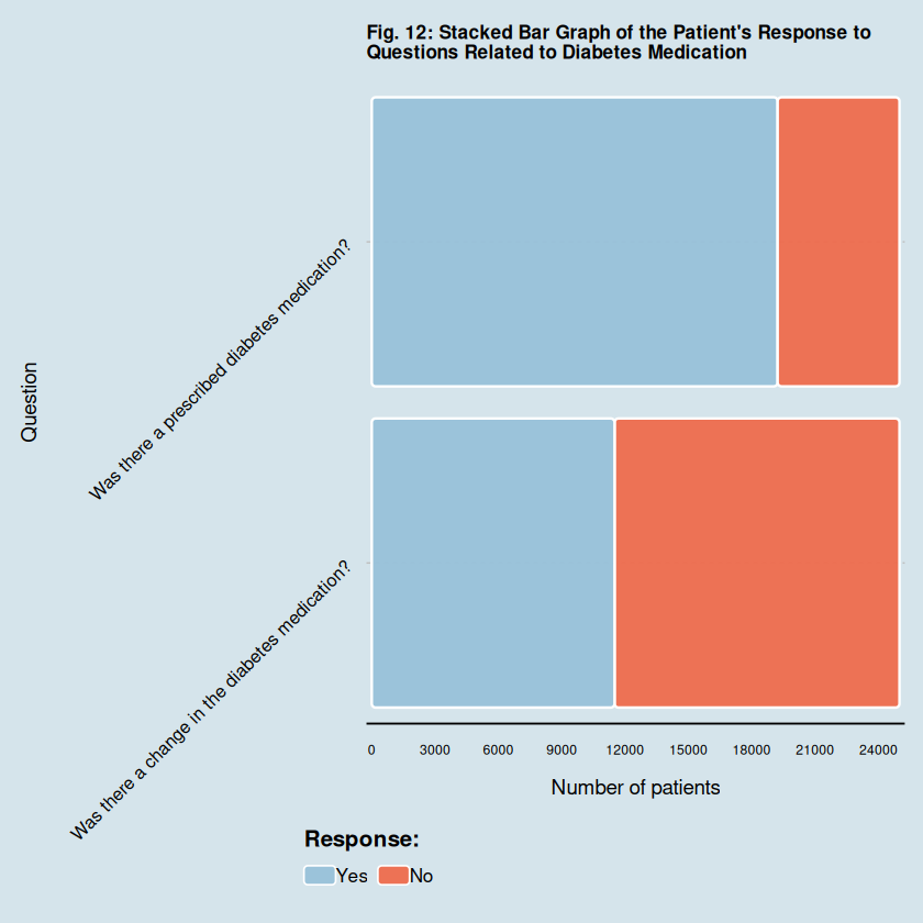
Among all the patients, 19,228 (76.91%) had been prescribed a diabetes medication, while 13,497 (53.99%) had not changed diabetes medication.
| Question | Response | Frequency | Percentage |
|---|---|---|---|
| Was there a change in the diabetes medication? | No | 13,497 | 53.99% |
| Was there a change in the diabetes medication? | Yes | 11,503 | 46.01% |
| Was there a prescribed diabetes medication? | Yes | 19,228 | 76.91% |
| Was there a prescribed diabetes medication? | No | 5,772 | 23.09% |
# Frequency Table
diab_ques_tbl <- readmissions %>%
  select(change, diabetes_med) %>%
  rename(
    `Was there a change in the diabetes medication?` = change,
    `Was there a prescribed diabetes medication?` = diabetes_med
  ) %>%
  pivot_longer(
    cols = everything(),
    names_to = "diab_ques",
    values_to = "response"
  ) %>%
  group_by(diab_ques, response) %>%
  summarize(n = n(), .groups = "drop_last") %>%
  mutate(perc = n / sum(n)) %>%
  ungroup() %>%
  arrange(diab_ques, desc(n)) %>%
  mutate(perc = label_percent(accuracy = 0.01)(perc))

# Fig. 12
diab_ques_stacked_bar_plot <- ggplot(diab_ques_tbl) +
  geom_chicklet(aes(x = fct_reorder(diab_ques, n), y = n,
                      fill = fct_reorder(response, n)),
                  color="white",
                  alpha=0.95,
                  radius = grid::unit(0.75, "mm"),
                  position="stack") +
  coord_flip() +
    scale_fill_manual(values = c("#EE6C4D", "#98C1D9"),
                      labels = c("No", "Yes")
                     ) +
  ggtitle("Fig. 12: Stacked Bar Graph of the Patient's Response to\nQuestions Related to Diabetes Medication\n") +
  labs(x="Question\n", y="\nNumber of patients", fill="Response:  ") +
  theme_economist() +
  scale_color_economist() +
    guides(fill = guide_legend(ncol=2,
                               reverse = TRUE,
                               override.aes = list(shape = 15,
                                                   size = 4),
                               title.position="top")) +
  theme(legend.position="bottom",
          legend.text = element_text(margin = margin(r = 2, unit = "pt"),
                                     size = 10),
          legend.title = element_text(face="bold",
                                      size = 12),
          axis.ticks = element_blank(),
          axis.text.y = element_text(size = 9.5, angle = 45, hjust = 1),
          axis.text.x = element_text(size=7.0),
          panel.grid.minor = element_blank(),
          panel.grid.major = element_line(color="grey",
                                          linetype="dashed",
                                          linewidth=0.3),
          plot.title = element_text(hjust = 0,
                                    size= 10),
          legend.box.margin = margin(t=0, b=0, l=-290, unit='pt')) +
  scale_y_continuous(expand = c(0.01, 0),
                   limits = c(),
                       breaks = seq(0, 25000, by=3000)) +
  scale_x_discrete(expand = c(0.5, 0))
2.1.2.5. Readmission
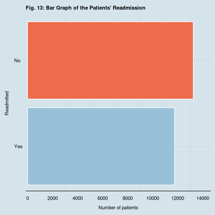
A slightly higher number of patients were not readmitted to the hospital compared to those who were readmitted. The blue bar represents the number of patients who were readmitted, which is 11,754 (47.02%), while the orange bar represents the number of patients who were not readmitted, which is 13,246 (52.98%)
| Readmitted | Frequency | Percentage |
|---|---|---|
| No | 13,246 | 52.98% |
| Yes | 11,754 | 47.02% |
# Frequency table
readmitted_fdt <- readmissions %>%
  select(readmitted) %>%
  group_by(readmitted) %>%
  count() %>%
  ungroup() %>%
  mutate(perc = label_percent(accuracy=0.01)(n/sum(n))) %>%
  arrange(desc(n))

# Fig. 13
readmitted_bar_plot <- ggplot(readmitted_fdt) +
  geom_chicklet(aes(x = fct_reorder(readmitted,n),
                      y = n),
                   fill=c("#EE6C4D", "#98C1D9"),
                  color="white",
                  radius = grid::unit(1, "mm"), position="stack") +
  coord_flip() +
  ggtitle("Fig. 13: Bar Graph of the Patients' Readmission \n") +
  labs(y="\nNumber of patients", x="Readmitted\n") +
  theme_economist() +
  scale_color_economist() +
  theme(legend.position="bottom",
          legend.text = element_text(margin = margin(r = 2, unit = "pt"),
                                     size = 10),
          axis.ticks = element_blank(),
          legend.title = element_text(face="bold",
                                      size = 12),
          panel.grid.minor = element_line(color="grey",
                                          linetype="dashed",
                                          linewidth=0.3),
      panel.grid.major = element_line(color="grey",
                                          linetype="dashed",
                                          linewidth=0.3),
          plot.title = element_text(hjust = 0,
                                    size= 12),
          legend.box.margin = margin(t=0, b=0, l=-95, unit='pt'))  +
  scale_y_continuous(expand = c(0.01, 0),
                       limits = c(0, 14500),
                       breaks = seq(0, 14500, by=2000)) +
  scale_x_discrete(expand = c(0.52, 0),
           labels = c("Yes", "No"))
2.2. Correlation Analysis
In this section, the patient readmission were analyzed by feature through contingency tables, graphs, and regression results.
As previously mentioned, the number of readmitted patients is 11,754 which translates to an overall readmission rate of 47.02%.
The table below shows the comparisons of means and medians of the readmitted, not readmitted, and overall patients in terms of the seven (7) numeric features. We can see that the three sets seem to be the same in characteristics.
# Summary statistics for numerical variables of readmitted patients
readmitted_sum_stats <- data.frame(
    Variable = readmissions %>%
    select_if(is.numeric) %>%
    colnames) %>%
  bind_cols(as.data.frame(t(readmissions %>% filter(readmitted == "yes") %>%
                              summarise_if(is.numeric, list(mean)) %>%
                              bind_rows(readmissions %>% filter(readmitted == "yes") %>%
                                          summarise_if(is.numeric, list(sd)),
                                        readmissions %>% filter(readmitted == "yes") %>%
                                          summarise_if(is.numeric, list(min)),
                                        readmissions %>% filter(readmitted == "yes") %>%
                                          summarise_if(is.numeric, list(median)),
                                        readmissions %>% filter(readmitted == "yes") %>%
                                          summarise_if(is.numeric, list(max)))
                             )) %>%
              rename(Mean = V1,
                     `Std. Dev.` = V2,
                     `Min.` = V3,
                     `Median` = V4,
                     `Max.` = V5))

rownames(readmitted_sum_stats) <- 1: nrow(readmitted_sum_stats)

# Summary statistics for numerical variables of not readmitted patients
not_readmitted_sum_stats <- data.frame(
    Variable = readmissions %>%
    select_if(is.numeric) %>%
    colnames) %>%
  bind_cols(as.data.frame(t(readmissions %>% filter(readmitted == "no") %>%
                              summarise_if(is.numeric, list(mean)) %>%
                              bind_rows(readmissions %>% filter(readmitted == "no") %>%
                                          summarise_if(is.numeric, list(sd)),
                                        readmissions %>% filter(readmitted == "no") %>%
                                          summarise_if(is.numeric, list(min)),
                                        readmissions %>% filter(readmitted == "no") %>%
                                          summarise_if(is.numeric, list(median)),
                                        readmissions %>% filter(readmitted == "no") %>%
                                          summarise_if(is.numeric, list(max)))
                             )) %>%
              rename(Mean = V1,
                     `Std. Dev.` = V2,
                     `Min.` = V3,
                     `Median` = V4,
                     `Max.` = V5))

rownames(not_readmitted_sum_stats) <- 1: nrow(not_readmitted_sum_stats)

# Med
readmitted_sum_stats %>%
  select(Variable, Mean, Median) %>%
  rename(readm_Mean = Mean, readm_Median = Median) %>%
    bind_cols(not_readmitted_sum_stats %>%
            select(Mean, Median) %>%
            rename(not_readm_Mean = Mean, not_readm_Median = Median),
          sum_stats %>%
            select(Mean, Median) %>%
            rename(overall_Mean = Mean, overall_Median = Median)
         )
| Variable | readm_Mean | readm_Median | not_readm_Mean | not_readm_Median | overall_Mean | overall_Median |
|---|---|---|---|---|---|---|
| <chr> | <dbl> | <dbl> | <dbl> | <dbl> | <dbl> | <dbl> |
| time_in_hospital | 4.5907776 | 4 | 4.3313453 | 4 | 4.45332 | 4 |
| n_lab_procedures | 43.9344053 | 45 | 42.6252454 | 44 | 43.24076 | 44 |
| n_procedures | 1.2713970 | 1 | 1.4242035 | 1 | 1.35236 | 1 |
| n_medications | 16.5678918 | 16 | 15.9724445 | 15 | 16.25240 | 15 |
| n_outpatient | 0.4875787 | 0 | 0.2588706 | 0 | 0.36640 | 0 |
| n_inpatient | 0.8816573 | 0 | 0.3801902 | 0 | 0.61596 | 0 |
| n_emergency | 0.2745448 | 0 | 0.1085611 | 0 | 0.18660 | 0 |
#readmissions %>%
#	group_by(readmitted) %>%
#	summarize(count = n(),
#			  median = median(time_in_hospital, na.rm = TRUE),
#			  IQR = IQR(time_in_hospital, na.rm = TRUE))

#ggboxplot(readmissions, x = "readmitted", y = "time_in_hospital",
#          color = "readmitted", palette = c("#FFA500", "#FF0000"),
#          ylab = "times_in_hospital", xlab = "readmitted?")

wilcox.test(time_in_hospital ~ readmitted,
                   data = readmissions,
                   exact = FALSE)

wilcox.test(n_procedures ~ readmitted,
                   data = readmissions,
                   exact = FALSE)

wilcox.test(n_lab_procedures ~ readmitted,
                   data = readmissions,
                   exact = FALSE)

wilcox.test(n_medications ~ readmitted,
                   data = readmissions,
                   exact = FALSE)

wilcox.test(n_outpatient ~ readmitted,
                   data = readmissions,
                   exact = FALSE)

wilcox.test(n_inpatient ~ readmitted,
                   data = readmissions,
                   exact = FALSE)

wilcox.test(n_emergency ~ readmitted,
                   data = readmissions,
                   exact = FALSE)
  Wilcoxon rank sum test with continuity correction

data:  time_in_hospital by readmitted
W = 73042702, p-value < 2.2e-16
alternative hypothesis: true location shift is not equal to 0


  Wilcoxon rank sum test with continuity correction

data:  n_procedures by readmitted
W = 81897160, p-value = 5.333e-14
alternative hypothesis: true location shift is not equal to 0


  Wilcoxon rank sum test with continuity correction

data:  n_lab_procedures by readmitted
W = 74776296, p-value = 6.973e-08
alternative hypothesis: true location shift is not equal to 0


  Wilcoxon rank sum test with continuity correction

data:  n_medications by readmitted
W = 71996398, p-value < 2.2e-16
alternative hypothesis: true location shift is not equal to 0


  Wilcoxon rank sum test with continuity correction

data:  n_outpatient by readmitted
W = 70962944, p-value < 2.2e-16
alternative hypothesis: true location shift is not equal to 0


  Wilcoxon rank sum test with continuity correction

data:  n_inpatient by readmitted
W = 61536228, p-value < 2.2e-16
alternative hypothesis: true location shift is not equal to 0


  Wilcoxon rank sum test with continuity correction

data:  n_emergency by readmitted
W = 72302580, p-value < 2.2e-16
alternative hypothesis: true location shift is not equal to 0
The table below shows the readmissions and rates by category of each factor arranged descendingly.
#
readmitted_age <- as.data.frame(xtabs(~ readmitted + age, data = readmissions)) %>%
  filter(readmitted == "yes") %>%
  group_by(age) %>%
  summarize(readmissions=sum(Freq), rate=sum(Freq)/25000, .groups = "keep") %>%
  arrange(desc(readmissions)) %>%
  ungroup()

#
readmitted_medical_specialty <- as.data.frame(xtabs(~ readmitted + medical_specialty, data = readmissions)) %>%
  filter(readmitted == "yes") %>%
  group_by(medical_specialty) %>%
  summarize(readmissions=sum(Freq), rate=sum(Freq)/25000, .groups = "keep") %>%
  arrange(desc(readmissions)) %>%
  ungroup()

#
readmitted_diag_1 <- as.data.frame(xtabs(~ readmitted + diag_1, data = readmissions)) %>%
  filter(readmitted == "yes") %>%
  group_by(diag_1) %>%
  summarize(readmissions=sum(Freq), rate=sum(Freq)/25000, .groups = "keep") %>%
  arrange(desc(readmissions)) %>%
  ungroup()

#
readmitted_diag_2 <- as.data.frame(xtabs(~ readmitted + diag_2, data = readmissions)) %>%
  filter(readmitted == "yes") %>%
  group_by(diag_2) %>%
  summarize(readmissions=sum(Freq), rate=sum(Freq)/25000, .groups = "keep") %>%
  arrange(desc(readmissions)) %>%
  ungroup()

#
readmitted_diag_3 <- as.data.frame(xtabs(~ readmitted + diag_3, data = readmissions)) %>%
  filter(readmitted == "yes") %>%
  group_by(diag_3) %>%
  summarize(readmissions=sum(Freq), rate=sum(Freq)/25000, .groups = "keep") %>%
  arrange(desc(readmissions)) %>%
  ungroup()

#
readmitted_glucose_test <- as.data.frame(xtabs(~ readmitted + glucose_test, data = readmissions)) %>%
  filter(readmitted == "yes") %>%
  group_by(glucose_test) %>%
  summarize(readmissions=sum(Freq), rate=sum(Freq)/25000, .groups = "keep") %>%
  arrange(desc(readmissions)) %>%
  ungroup()

#
readmitted_A1Ctest <- as.data.frame(xtabs(~ readmitted + A1Ctest, data = readmissions)) %>%
  filter(readmitted == "yes") %>%
  group_by(A1Ctest) %>%
  summarize(readmissions=sum(Freq), rate=sum(Freq)/25000, .groups = "keep") %>%
  arrange(desc(readmissions)) %>%
  ungroup()

#
readmitted_change <- as.data.frame(xtabs(~ readmitted + change, data = readmissions)) %>%
  filter(readmitted == "yes") %>%
  group_by(change) %>%
  summarize(readmissions=sum(Freq), rate=sum(Freq)/25000, .groups = "keep") %>%
  arrange(desc(readmissions)) %>%
  ungroup()

#
readmitted_diabetes_med <- as.data.frame(xtabs(~ readmitted + diabetes_med, data = readmissions)) %>%
  filter(readmitted == "yes") %>%
  group_by(diabetes_med) %>%
  summarize(readmissions=sum(Freq), rate=sum(Freq)/25000, .groups = "keep") %>%
  arrange(desc(readmissions)) %>%
  ungroup()

#
readmitted_factor <- rbind(readmitted_age %>% rename(category = age) %>% mutate(factor = "age"),
  readmitted_medical_specialty %>% rename(category = medical_specialty) %>% mutate(factor = "medical_specialty"),
  readmitted_diag_1 %>% rename(category = diag_1) %>% mutate(factor = "diag_1"),
  readmitted_diag_2 %>% rename(category = diag_2) %>% mutate(factor = "diag_2"),
  readmitted_diag_3 %>% rename(category = diag_3) %>% mutate(factor = "diag_3"),
  readmitted_glucose_test %>% rename(category = glucose_test) %>% mutate(factor = "glucose_test"),
  readmitted_A1Ctest %>% rename(category = A1Ctest) %>% mutate(factor = "A1Ctest"),
  readmitted_change %>% rename(category = change) %>% mutate(factor = "change"),
  readmitted_diabetes_med %>% rename(category = diabetes_med) %>% mutate(factor = "diabetes_med")
)

readmitted_factor %>%
  select(factor, everything())
| factor | category | readmissions | rate |
|---|---|---|---|
| <chr> | <fct> | <int> | <dbl> |
| age | [70-80) | 3336 | 0.13344 |
| age | [60-70) | 2770 | 0.11080 |
| age | [80-90) | 2239 | 0.08956 |
| age | [50-60) | 1966 | 0.07864 |
| age | [40-50) | 1127 | 0.04508 |
| age | [90-100) | 316 | 0.01264 |
| medical_specialty | InternalMedicine | 1596 | 0.06384 |
| medical_specialty | Other | 1105 | 0.04420 |
| medical_specialty | Family/GeneralPractice | 932 | 0.03728 |
| medical_specialty | Emergency/Trauma | 931 | 0.03724 |
| medical_specialty | Cardiology | 634 | 0.02536 |
| medical_specialty | Surgery | 500 | 0.02000 |
| medical_specialty | Missing | 0 | 0.00000 |
| diag_1 | Circulatory | 3750 | 0.15000 |
| diag_1 | Other | 2932 | 0.11728 |
| diag_1 | Respiratory | 1806 | 0.07224 |
| diag_1 | Digestive | 1105 | 0.04420 |
| diag_1 | Diabetes | 937 | 0.03748 |
| diag_1 | Injury | 727 | 0.02908 |
| diag_1 | Musculoskeletal | 495 | 0.01980 |
| diag_1 | Missing | 0 | 0.00000 |
| diag_2 | Other | 4248 | 0.16992 |
| diag_2 | Circulatory | 3932 | 0.15728 |
| diag_2 | Respiratory | 1406 | 0.05624 |
| diag_2 | Diabetes | 1283 | 0.05132 |
| diag_2 | Digestive | 431 | 0.01724 |
| diag_2 | Injury | 240 | 0.00960 |
| diag_2 | Musculoskeletal | 197 | 0.00788 |
| diag_2 | Missing | 0 | 0.00000 |
| diag_3 | Other | 4253 | 0.17012 |
| diag_3 | Circulatory | 3712 | 0.14848 |
| diag_3 | Diabetes | 1947 | 0.07788 |
| diag_3 | Respiratory | 954 | 0.03816 |
| diag_3 | Digestive | 430 | 0.01720 |
| diag_3 | Musculoskeletal | 205 | 0.00820 |
| diag_3 | Injury | 197 | 0.00788 |
| diag_3 | Missing | 0 | 0.00000 |
| glucose_test | no | 11064 | 0.44256 |
| glucose_test | high | 357 | 0.01428 |
| glucose_test | normal | 333 | 0.01332 |
| A1Ctest | no | 9935 | 0.39740 |
| A1Ctest | high | 1299 | 0.05196 |
| A1Ctest | normal | 520 | 0.02080 |
| change | no | 6077 | 0.24308 |
| change | yes | 5677 | 0.22708 |
| diabetes_med | yes | 9367 | 0.37468 |
| diabetes_med | no | 2387 | 0.09548 |
2.3. Logistic Regression
2.3.1. Model
Since the feature representing a patient’s readmission takes on two values, ‘yes’ or ‘no’, it is used as the dependent variable of a multivariate logistic regression model in order to predict the odds of readmission. Also, not all of the patient’s features are used as independent variables, that is, variables medical_specialty, glucose_test, and A1Ctest were excluded due to large number of missing values. Variables with few missing values (diag_1, diag_2, and diag_3) were imputed by their respective modes.
The reference category for each factor variable is:
- age: [40-50)
- diag_1, diag_2, and diag_3: Circulatory
- change: no
- diabetes_med: no
Below are the estimates of the coefficients along with their standard errors, t-statistics, p-values, odds ratios (ORs), and 95% CIs of the ORs.
## Univariate Regression Analysis
logstc_model_age <- glm(readmitted ~ age, data=readmissions, family="binomial"(link=logit))

logstc_model_time_in_hospital <- glm(readmitted ~ time_in_hospital, data=readmissions, family="binomial"(link=logit))

logstc_model_n_procedures <- glm(readmitted ~ n_procedures, data=readmissions, family="binomial"(link=logit))

logstc_model_n_lab_procedures <- glm(readmitted ~ n_lab_procedures, data=readmissions, family="binomial"(link=logit))

logstc_model_n_medications <- glm(readmitted ~ n_medications, data=readmissions, family="binomial"(link=logit))

logstc_model_n_outpatient <- glm(readmitted ~ n_outpatient, data=readmissions, family="binomial"(link=logit))

logstc_model_n_inpatient <- glm(readmitted ~ n_inpatient, data=readmissions, family="binomial"(link=logit))

logstc_model_n_emergency <- glm(readmitted ~ n_emergency, data=readmissions, family="binomial"(link=logit))

logstc_model_medical_specialty <- glm(readmitted ~ medical_specialty, data=readmissions, family="binomial"(link=logit))

logstc_model_diag_1 <- glm(readmitted ~ diag_1, data=readmissions, family="binomial"(link=logit))

logstc_model_diag_2 <- glm(readmitted ~ diag_2, data=readmissions, family="binomial"(link=logit))

logstc_model_diag_3 <- glm(readmitted ~ diag_3, data=readmissions, family="binomial"(link=logit))

logstc_model_change <- glm(readmitted ~ change, data=readmissions, family="binomial"(link=logit))

logstc_model_diabetes_med <- glm(readmitted ~ diabetes_med, data=readmissions, family="binomial"(link=logit))

# Install and load the "questionr" package
# For calculating the odds ratio
suppressWarnings(suppressMessages(install.packages("questionr")))
suppressPackageStartupMessages(library(questionr))

#
#as.data.frame(summary.lm(logstc_model_age)$coefficients) %>%
#	rownames_to_column("Variable") %>%
#	mutate(`Signif. Code` = case_when(`Pr(>|t|)` < 0.001 ~  "***",
#                                      `Pr(>|t|)` >= 0.001 & `Pr(>|t|)` < 0.01 ~ "**",
#                                      `Pr(>|t|)` >= 0.01 & `Pr(>|t|)` < 0.05 ~ "*",
#                                      `Pr(>|t|)` >= 0.05 & `Pr(>|t|)` < 0.1 ~ ".",
#                                       TRUE ~ "")) %>%
#	merge(odds.ratio(logstc_model_age, 0.95) %>%
#		  	rownames_to_column("Variable") %>%
#		  	select(-p))

# Create mode() function to calculate mode
mode <- function(x, na.rm = FALSE) {
  if(na.rm){ #if na.rm is TRUE, remove NA values from input x
    x = x[!is.na(x)]
  }
  val <- unique(x)
  return(val[which.max(tabulate(match(x, val)))])
}


## Multivariate Regression Analysis

data_for_regression <- readmissions %>%
  select(-c(medical_specialty, glucose_test, A1Ctest)) %>%
  mutate_all(~case_when(is.character(.) & is.na(.) ~ mode(.),
              TRUE ~ .))

# Logistics Regression Model
logstc_model <- glm(readmitted ~ ., data=data_for_regression, family="binomial"(link=logit))

# Summary statistics of the full model
#paste("Residual standard error:", round(summary.lm(full_model)$sigma, 4),
#      " ,  R-square: ", round(summary.lm(full_model)$r.squared, 4),
#      " ,  Adj. R-square: ", round(summary.lm(full_model)$adj.r.squared, 4))

# Full model's table of estimated coefficients, their SEs, t-stats, and (two-sided) p-values
summary_logstc <- as.data.frame(summary.lm(logstc_model)$coefficients) %>%
  rownames_to_column("Variable") %>%
  mutate(`Signif. Code` = case_when(`Pr(>|t|)` < 0.001 ~  "***",
                                      `Pr(>|t|)` >= 0.001 & `Pr(>|t|)` < 0.01 ~ "**",
                                      `Pr(>|t|)` >= 0.01 & `Pr(>|t|)` < 0.05 ~ "*",
                                      `Pr(>|t|)` >= 0.05 & `Pr(>|t|)` < 0.1 ~ ".",
                                       TRUE ~ "")) %>%
  merge(odds.ratio(logstc_model, 0.95) %>%
        rownames_to_column("Variable") %>%
        select(-p))
Waiting for profiling to be done...
summary_logstc
| Variable | Estimate | Std. Error | t value | Pr(>|t|) | Signif. Code | OR | 2.5 % | 97.5 % |
|---|---|---|---|---|---|---|---|---|
| <chr> | <dbl> | <dbl> | <dbl> | <dbl> | <chr> | <dbl> | <dbl> | <dbl> |
| (Intercept) | -0.676308664 | 0.0727457345 | -9.29688413 | 1.562023e-20 | *** | 0.5084905 | 0.4433359 | 0.5830338 |
| age[50-60) | 0.027580089 | 0.0552481797 | 0.49920358 | 6.176404e-01 | 1.0279639 | 0.9264833 | 1.1407389 | |
| age[60-70) | 0.140138815 | 0.0531046658 | 2.63891718 | 8.322339e-03 | ** | 1.1504335 | 1.0410870 | 1.2715419 |
| age[70-80) | 0.208365868 | 0.0523118146 | 3.98315122 | 6.820194e-05 | *** | 1.2316637 | 1.1162713 | 1.3593055 |
| age[80-90) | 0.220960379 | 0.0559845407 | 3.94681061 | 7.941792e-05 | *** | 1.2472740 | 1.1226112 | 1.3860596 |
| age[90-100) | -0.053054919 | 0.0918668717 | -0.57751960 | 5.635938e-01 | 0.9483279 | 0.7973616 | 1.1269743 | |
| changeyes | 0.039509849 | 0.0325303449 | 1.21455365 | 2.245480e-01 | 1.0403007 | 0.9785075 | 1.1060109 | |
| diabetes_medyes | 0.227533505 | 0.0381635967 | 5.96205611 | 2.524595e-09 | *** | 1.2554995 | 1.1685024 | 1.3490779 |
| diag_1Diabetes | 0.148048457 | 0.0612105412 | 2.41867584 | 1.558428e-02 | * | 1.1595691 | 1.0334018 | 1.3012846 |
| diag_1Digestive | -0.013140042 | 0.0542553278 | -0.24218898 | 8.086357e-01 | 0.9869459 | 0.8910678 | 1.0930423 | |
| diag_1Injury | -0.188171950 | 0.0606963642 | -3.10021782 | 1.935954e-03 | ** | 0.8284722 | 0.7388791 | 0.9286184 |
| diag_1Musculoskeletal | -0.227602478 | 0.0693867245 | -3.28020207 | 1.038761e-03 | ** | 0.7964408 | 0.6986402 | 0.9072697 |
| diag_1Other | -0.166568633 | 0.0393675922 | -4.23111052 | 2.333769e-05 | *** | 0.8465647 | 0.7860692 | 0.9116689 |
| diag_1Respiratory | -0.037630283 | 0.0451369154 | -0.83369195 | 4.044626e-01 | 0.9630689 | 0.8845903 | 1.0484649 | |
| diag_2Diabetes | -0.051929157 | 0.0495084120 | -1.04889564 | 2.942364e-01 | 0.9493961 | 0.8648507 | 1.0420843 | |
| diag_2Digestive | -0.155934654 | 0.0775036909 | -2.01196423 | 4.423453e-02 | * | 0.8556151 | 0.7391957 | 0.9897442 |
| diag_2Injury | -0.178988923 | 0.0948599735 | -1.88687511 | 5.918882e-02 | . | 0.8361152 | 0.6987815 | 0.9989114 |
| diag_2Musculoskeletal | -0.033857049 | 0.1107840497 | -0.30561303 | 7.599019e-01 | 0.9667097 | 0.7842180 | 1.1904138 | |
| diag_2Other | -0.077084024 | 0.0351261254 | -2.19449266 | 2.820927e-02 | * | 0.9258121 | 0.8665632 | 0.9891005 |
| diag_2Respiratory | -0.065264765 | 0.0477940091 | -1.36554279 | 1.720949e-01 | 0.9368194 | 0.8561699 | 1.0249865 | |
| diag_3Diabetes | -0.046963422 | 0.0423694828 | -1.10842565 | 2.676888e-01 | 0.9541223 | 0.8809486 | 1.0333233 | |
| diag_3Digestive | -0.001843499 | 0.0777562600 | -0.02370869 | 9.810852e-01 | 0.9981582 | 0.8620371 | 1.1553276 | |
| diag_3Injury | -0.120078026 | 0.1048401374 | -1.14534403 | 2.520777e-01 | 0.8868512 | 0.7273160 | 1.0795854 | |
| diag_3Musculoskeletal | -0.078950919 | 0.1062193390 | -0.74328197 | 4.573180e-01 | 0.9240853 | 0.7560518 | 1.1280833 | |
| diag_3Other | -0.079470675 | 0.0342788439 | -2.31835925 | 2.043791e-02 | * | 0.9236051 | 0.8658785 | 0.9851707 |
| diag_3Respiratory | -0.005092567 | 0.0554708711 | -0.09180615 | 9.268528e-01 | 0.9949204 | 0.8962213 | 1.1044124 | |
| n_emergency | 0.216328283 | 0.0264002294 | 8.19418195 | 2.643943e-16 | *** | 1.2415099 | 1.1822193 | 1.3057433 |
| n_inpatient | 0.383827889 | 0.0150281702 | 25.54056032 | 4.841353e-142 | *** | 1.4678928 | 1.4272055 | 1.5102947 |
| n_lab_procedures | 0.001063578 | 0.0007531879 | 1.41210218 | 1.579325e-01 | 1.0010641 | 0.9996458 | 1.0024849 | |
| n_medications | 0.001389491 | 0.0021909349 | 0.63420012 | 5.259561e-01 | 1.0013905 | 0.9972669 | 1.0055284 | |
| n_outpatient | 0.120890635 | 0.0137120597 | 8.81637317 | 1.258480e-18 | *** | 1.1285015 | 1.1000870 | 1.1583729 |
| n_procedures | -0.043869470 | 0.0091983519 | -4.76927502 | 1.859425e-06 | *** | 0.9570789 | 0.9406329 | 0.9737829 |
| time_in_hospital | 0.017843737 | 0.0054244633 | 3.28949358 | 1.005080e-03 | ** | 1.0180039 | 1.0076614 | 1.0284549 |
2.3.2. Odds Ratio
To interpret the odds ratios in the model, we will separate them into categorical and numerical variables once more.
The odds ratio for categorical data is the percentage increase (or decrease) in the odds of readmission among patients within a particular case-category compared to those in the control or reference group. Therefore:
- Patients in the [80-90], [70-80], and [60-70] age groups have 24.73%, 23.17%, and 15.04% higher odds of readmission, respectively, than those in the [40-50] group.
- Patients with diabetes as their primary diagnosis had a 15.96% greater odds of readmission than those with a circulatory diagnosis. On the other hand, those with a secondary and additional secondary diagnosis of diabetes had a 5.06% and 4.59% decrease, respectively, as compared to those with circulatory.
- Patients who were prescribed a diabetes medication had a 25.55% increase in the odds of readmission as compared to those without.
The odds ratio for numerical variables is the percentage increase (or decrease) in the odds of readmission for every unit increase (or decrease) in that variable. Therefore,
- Every additional hospital day increases the odds of a patient’s readmission by 1.8%.
- An increase in the number of procedures performed during a patient’s hospital stay reduces the odds of readmission by 4.29%.
- With every increase in the number of outpatient, inpatient, and emergency department visits prior to hospitalization, the odds of readmission rise by 46.79%, 12.85%, and 24.15%, respectively.
3. Recommendations
Using the odds ratios of the multivariate logistic model, the following groups should be the hospital’s focus for their follow up efforts to better monitor patients with high probability of readmission:
- Individuals that are at least 60 but below 90 years of age at the time of admission.
- Primarily diagnosed with diabetes or was prescribed a diabetes medication.
- With either of the following characteristics: long hospitalization time or frequently visited before hospital stay for all either types (outpatient, inpatient, and emergency room).
Nevertheless, it is also advised to explore for additional characteristics that can help better predict the probability of readmission among patients, as the data used may be insufficient to reliably identify patient groups with the best readmission rates.
4. Reference
Mahto, A. (2013, September 21). Answer to “How to calculate the median on grouped dataset?” Stack Overflow. http://stackoverflow.com/a/18931054/1270695
Strack, B., DeShazo, J. P., Gennings, C., Olmo, J. L., Ventura, S., Cios, K. J., & Clore, J. N. (2014). Impact of HbA1c measurement on hospital readmission rates: Analysis of 70,000 clinical database patient records. BioMed Research International, 2014, 781670, 11 pages. https://doi.org/10.1155/2014/781670