
Manhattan’s Urban Forestry Report, 2015
Manhattan’s Urban Forestry Report, 2015

0. Executive Summary
Based on the data and results, the tree population and species present in Manhattan, NYC, can be summarized as follows:
- Greater numbers of trees are most likely to be found in neighborhoods with larger plots of land.
- The majority of the trees in Manhattan are on-curb, with only a few that are offset from the curb.
- The majority of the trees in Manhattan are alive and in fair to good health, while only a small number are dead and in poor health.
- Although specific root, trunk, and branch problems are not of significant concerns, few of the trees are affected by paving stones in the tree bed (a kind of root problem) as well as other unspecified trunk and branch problems.
- Manhattan has a rich and diverse set of tree species.
The species recommendation for tree planting in Manhattan’s streets is a combination of some of the borough’s highly and averagely abundant species that have shown favorable qualities of size and health. Specifically, the following are the five species that are highly recommended:
- Siberian elm
- Willow oak
- Honeylocust
- American elm
- Pin oak
1. Background
1.1. Introduction
The urban design team believes that tree size (in terms of trunk diameter) and health are the most desirable characteristics of city trees. In order to help the planning department improve the quantity and quality of trees in New York City, our organization is advised to provide a data analysis report.
1.2. Objectives
The main objective of this report is to profile Manhattan’s tree population and species by different attributes using summary statistics, visualizations, and textual explanations. Specifically, it aims to:
- Describe all censused trees by their spatial and biological characteristics.
- Map the tree profile of the neighborhoods.
- Illustrate the biodiversity and biology of the tree species in Manhattan.
- Determine tree species with the best traits.
1.3. Libraries
# Load required packages
library(tidyverse)
library(dplyr)
library(ggplot2)
library(sf)
library(geojsonsf)
library(geojsonio)
library(scales)
library(remotes)
library(rwantshue)
library(ggfun)
library(ggchicklet)
1.4. Datasets
The datasets presented below are sourced from the NYC Open Data provided by the City of New York.
# Read the 'trees' data set from the CSV file
trees <- read_csv("data/trees.csv", show_col_types=FALSE) %>%
  mutate(spc_common = str_to_sentence(spc_common))

# Read the 'neighborhoods' data set from the SHP file
neighborhoods <- st_read("data/nta.shp", quiet=TRUE) %>%
  select(boroname, ntacode, ntaname, geometry, shape_area)

# Create a merged data frame for the 'trees' and 'neighborhoods' data sets
merged_trees_and_neighborhoods <- trees %>%
  full_join(neighborhoods, by = c("nta"="ntacode", "nta_name"="ntaname"))

# Total number of censused trees (Population)
N_trees <- trees %>%
  summarize(total_number_of_censused_trees = n())
1.4.1. Trees
Based on the TreesCount! 2015 Street Tree Census, this dataset was collected by volunteers and staff organized by NYC Parks & Recreation, along with partner organizations. It includes information on tree species, diameter, and perceived health. Accompanying blockface data indicate the status of data collection and release across the city.
| Variable | Description |
|---|---|
| tree_id | Unique id of each tree |
| tree_dbh | The diameter of the tree in inches measured at 54 inches above the ground |
| curb_loc | Location of the tree bed in relation to the curb Either along the curb (OnCurb) or offset from the curb (OffsetFromCurb) |
| spc_common | Common name for the species |
| status | Indicates whether the tree is alive or standing dead |
| health | Indication of the tree’s health (Good, Fair, and Poor) |
| root_stone | Indicates the presence of a root problem caused by paving stones in the tree bed |
| root_grate | Indicates the presence of a root problem caused by metal grates in the tree bed |
| root_other | Indicates the presence of other root problems |
| trunk_wire | Indicates the presence of a trunk problem caused by wires or rope wrapped around the trunk |
| trnk_light | Indicates the presence of a trunk problem caused by lighting installed on the tree |
| trnk_other | Indicates the presence of other trunk problems |
| brch_light | Indicates the presence of a branch problem caused by lights or wires in the branches |
| brch_shoe | Indicates the presence of a branch problem caused by shoes in the branches |
| brch_other | Indicates the presence of other branch problems |
| postcode | Five-digit zip code where the tree is located |
| nta | Neighborhood Tabulation Area (NTA) code from the 2010 US Census for the tree |
| nta_name | Neighborhood name |
| latitude | Latitude of the tree in decimal degrees |
| longitude | Longitude of the tree in decimal degrees |
1.4.2. Neighborhoods
This dataset is based on the boundaries of Neighborhood Tabulation Areas (NTAs), created by the NYC Department of City Planning using whole census tracts from the 2010 Census as building blocks. These aggregations of census tracts form subsets of New York City’s 55 Public Use Microdata Areas (PUMAs).
| Variable | Description |
|---|---|
| ntacode | NTA code |
| ntaname | Neighborhood name |
| geometry | Polygon that defines the neighborhood |
2. Results & Discussion
2.1. Tree Population
Using descriptive and spatial analyses, the following information outlines the location and physical attributes of all Manhattan trees in 2015 with a population size (\(N\)) of 64,229:
2.1.1. Spatial
2.1.1.1. Tree Location by Neighborhood
# Top 10 NTAs in terms of shape size
top_nta_area <- neighborhoods %>%
  filter(boroname == "Manhattan", ntacode != "MN99") %>%
  arrange(desc(shape_area)) %>%
  slice(1:10)

# Tree count per neighborhood
nbh_tree_cnts <- merged_trees_and_neighborhoods %>%
  filter(boroname == "Manhattan", nta != "MN99") %>%
  group_by(nta, nta_name) %>%
  summarize(number_of_trees = n(), .groups="keep") %>%
  arrange(desc(number_of_trees)) %>%
  ungroup() %>%
  mutate(proportion = round(number_of_trees/sum(number_of_trees), digits = 4))

# Species richness per neighborhood
nbh_rchns <- trees %>%
  filter(!(spc_common=="null")) %>%
  group_by(nta, nta_name) %>%
  summarize(richness = n_distinct(spc_common), .groups="keep") %>%
  arrange(desc(richness)) %>%
  ungroup()

# Data for maps
nbhs_map <- nbh_tree_cnts %>%
  full_join(neighborhoods, c("nta"="ntacode", "nta_name"="ntaname")) %>%
  full_join(nbh_rchns, c("nta", "nta_name")) %>%
  mutate(borough = substr(nta, 1, 2),
         nta_code_and_name = paste(nta, nta_name, sep=": "),
         nta_and_tree_cnt = ifelse(number_of_trees < 1000,
                                   paste(nta,  " - ", "   ", prettyNum(number_of_trees,big.mark=","), " : ", nta_name, sep=""),
                                   paste(nta,  " - ", prettyNum(number_of_trees, big.mark=","), " : ", nta_name, sep="")
         ),
         nta_and_rchns = paste(nta,  " - ", prettyNum(richness, big.mark=","),
                               " : ", nta_name, sep="")
  ) %>%
  st_as_sf %>%
  st_transform("+proj=longlat +ellps=intl +no_defs +type=crs")

# Colorize the NTAs
color_scheme <- iwanthue(seed=1234, force_init=TRUE)
nta_colors <- color_scheme$hex(nrow(nbhs_map %>%  filter(borough == "MN")))

# Data of tree locations
tree_locs <- trees %>%
  st_as_sf(coords = c("longitude", "latitude"), crs=4326) %>%
  st_transform("+proj=longlat +ellps=intl +no_defs +type=crs")


# Map of tree locations by neighborhood
tree_locs_map_plot <- ggplot() +
  geom_sf(data = nbhs_map,
          fill="#E8EAED", color="grey") +
  stat_sf_coordinates(data = tree_locs,
                      aes(color = paste(nta, nta_name, sep=": ")),
                      size=0.001
  ) +
  stat_sf_coordinates(data = nbhs_map %>% filter(borough=="MN", nta!="MN99"),
                      color="grey25", size=0.25) +
  geom_sf(data = nbhs_map %>% filter(borough=="MN", nta!="MN99"),
          color="grey25",
          alpha=0.1) +
  theme(legend.position = c(0.024, 0.5),
        legend.justification=0.0,
        legend.key.width = unit(2.5, 'mm'),
        legend.key.height = unit(1.8, 'mm'),
        legend.direction="vertical",
        legend.background= element_roundrect(r = grid::unit(0.02, "snpc"),
                                             fill=alpha("#FFFFFF", 0.90)),
        legend.key = element_rect(fill=NA),
        legend.text = element_text(margin = margin(r=5, unit="pt"),
                                   color="#65707C",
                                   family="sans serif"),
        legend.title = element_text(face="bold",
                                    color="#65707C",
                                    size=8.5,
                                    family="sans serif"),
        axis.title = element_text(color="#65707C",
                                  face="bold",
                                  family="sans serif"),
        axis.text = element_text(color="#65707C",
                                 size=7,
                                 family="sans serif"),
        axis.text.x = element_text(angle=90,
                                   vjust=0.5,
                                   hjust=1),
        axis.line = element_line(colour="grey",
                                 linewidth=0.5),
        panel.grid.major = element_line(color="grey",
                                        linetype="dashed",
                                        linewidth=0.25),
        panel.border = element_rect(color="grey40",
                                    fill=NA),
        panel.spacing = unit(2, "lines"),
        panel.background  = element_roundrect(r = grid::unit(0.001, "snpc"),
                                              fill=alpha("#9CC0F9", 1)),
    rect = element_rect(fill = "transparent"),
        plot.title = element_text(color="#65707C",
                                  vjust=10,
                                  size=14,
                                  family="sans serif")) +
  labs(x="", y="", color="    Code: Name") +
  ggtitle("Fig. 1: Map of the Tree Locations by Neighborhood in Manhattan") +
  scale_x_continuous(limits = c(-74.25, -73.89),
                     breaks = seq(-74.25, -73.89, by=0.02)) +
  scale_y_continuous(limits = c(40.68, 40.88),
                     breaks = seq(40.68, 40.88, by=0.02)) +
  guides(color = guide_legend(ncol=1,
                              override.aes = list(shape=15,
                                                  size=2.5
                              ))) +
  ggrepel::geom_text_repel(data = nbhs_map %>% filter(borough == "MN", nta != "MN99"),
                            aes(label = nta, geometry = geometry),
                            stat="sf_coordinates",
                            min.segment.length=0,
                            size=2,
                            label.size=NA,
                fontface="bold"
              ) +
  coord_sf(xlim = c(-74.25, -73.89), ylim = c(40.68, 40.88)) +
  scale_color_manual(values = nta_colors)
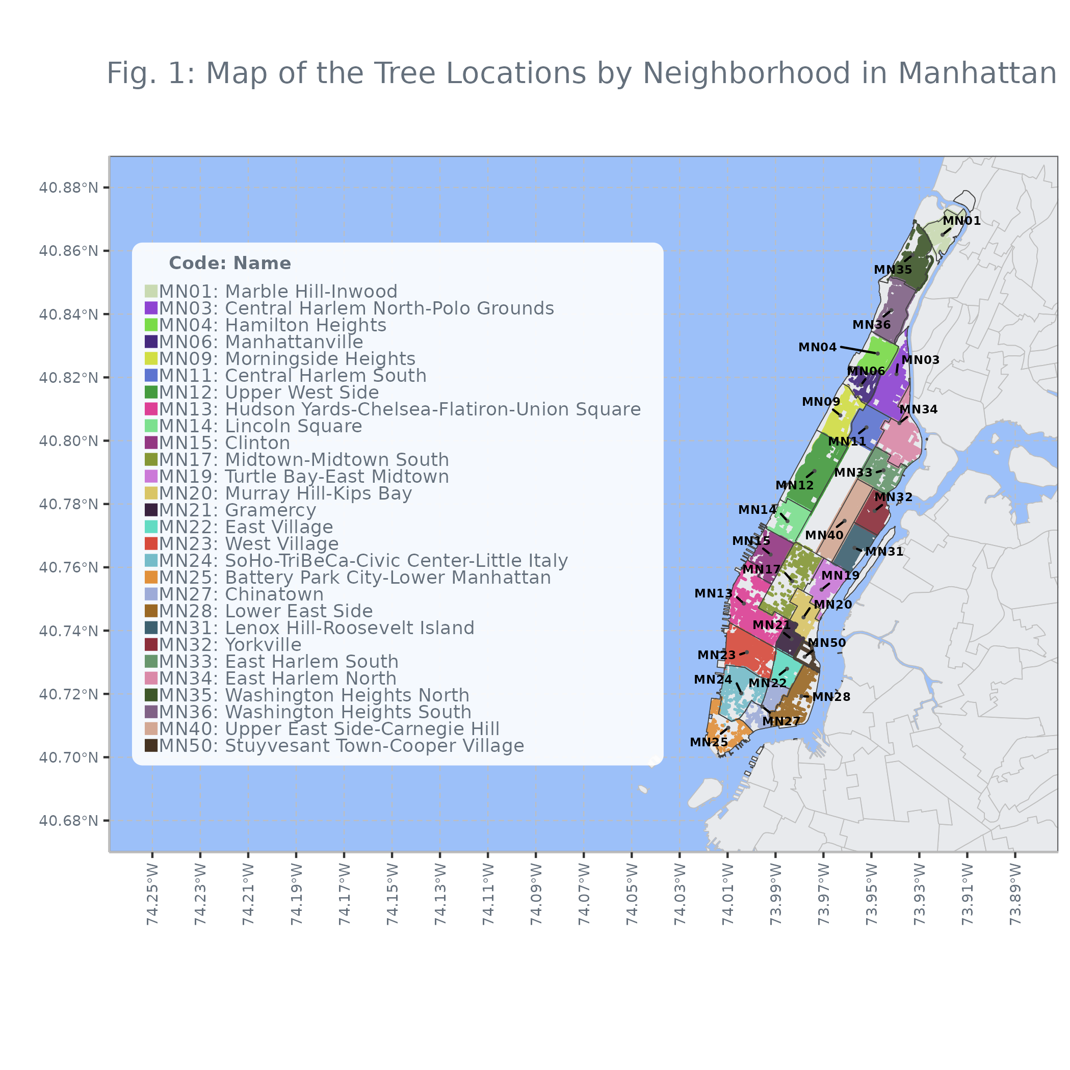
While trees seem to cover much each of Manhattan’s 28 neighborhoods, some of the southern ones, including MN13, MN17, MN24, MN25, MN27, MN28, and MN50, have empty areas. Interestingly, four of these aforementioned neighborhoods (indicated by *) are among the top ten in terms of shape size, which are:
- Hudson Yards-Chelsea-Flatiron-Union Square (MN13)*
- Upper West Side (MN12)
- Midtown-Midtown South (MN17)*
- Central Harlem North-Polo Grounds (MN03)
- West Village (MN23)
- SoHo-TriBeCa-Civic Center-Little Italy (MN24)*
- East Harlem North (MN34)
- Lower East Side (MN28)*
- Washington Heights South (MN36)
- Washington Heights North (MN35)
2.1.1.2. Tree Counts by Neighborhood
# Table for Top 10 Tree-Producing Neighborhoods
for_table_nbh_tree_cnts <- nbh_tree_cnts %>%
  slice(1:10) %>%
  rownames_to_column("rank") %>%
  mutate(number_of_trees = prettyNum(number_of_trees, big.mark=","),
           percentage = label_percent(accuracy=0.01)(proportion)) %>%
  select(-proportion)

# Order by number of trees
nbhs_map$nta_and_tree_cnt <- factor(
    nbhs_map$nta_and_tree_cnt,
       levels = nbhs_map$nta_and_tree_cnt,
       ordered=TRUE
)

# Map of NTAs' tree counts
nbhs_tree_cnts_map_plot <- ggplot() +
  geom_sf(data = nbhs_map %>% filter(borough != "MN" | nta == "MN99"),
            fill="#E8EAED", color="grey") +
  geom_sf(data = nbhs_map %>% filter(borough == "MN", nta != "MN99"),
            aes(fill = number_of_trees,
                color = nta_and_tree_cnt
           )) +
    stat_sf_coordinates(data = nbhs_map %>% filter(nta %in% for_table_nbh_tree_cnts$nta),
                        color="grey25", size=0.5) +
    theme(legend.position = #c(0.7, 0.8),
          c(0.369, 0.5),
          #c(0.025, 0.5),
          legend.justification=0.0,
          legend.key.width = unit(2.5, 'mm'),
        legend.key.height = unit(1.8, 'mm'),
          legend.direction="vertical",
          legend.background = element_roundrect(r = grid::unit(0.02, "snpc"),
                                               fill = alpha("#FFFFFF", 0.90)),
          legend.key = element_rect(fill=NA),
          legend.text = element_text(margin = margin(r=5, unit="pt"),
                                     size=7.9,
                                   color="#65707C",
                                     family="sans serif"),
          legend.title = element_text(face="bold",
                                      color="#65707C",
                                      size=8.5,
                                      family="sans serif"),
          axis.title = element_text(color="#65707C",
                                    face="bold",
                                    family="sans serif"),
          axis.text = element_text(color="#65707C",
                                   size=7,
                                   family="sans serif"),
          axis.text.x = element_text(angle=90,
                                     vjust=0.5,
                                     hjust=1),
          axis.line = element_line(colour="grey",
                                   linewidth=0.5),
          panel.grid.major = element_line(color="grey",
                                          linetype="dashed",
                                          linewidth=0.25),
          panel.border = element_rect(color="grey40",
                                      fill=NA),
          panel.spacing = unit(2, "lines"),
          panel.background  = element_roundrect(r = grid::unit(0.001, "snpc"),
                                               fill = alpha("#9CC0F9", 1)),
      rect = element_rect(fill = "transparent"),
          plot.title = element_text(color="#65707C",
                                    vjust=10,
                                    size=14,
                                    family="sans serif")) +
     labs(x="", y="", color="   Code - Number of trees : Name"
             ) +
     ggtitle("Fig. 2: Map of the Number of Trees in Manhattan's Neighborhoods") +
  scale_x_continuous(expand = c(0.01, 0),
                       limits = c(-74.04, -73.64),
                       breaks = seq(-74.04, -73.64, by=0.02)) +
  scale_y_continuous(expand = c(0.01, 0),
                       limits = c(40.68, 40.88),
                       breaks = seq(40.68, 40.88, by=0.02)) +
  scale_color_manual(values = replicate(28, "grey25")) +
  scale_fill_gradient2(low = muted("499F78"),
                         high = muted("#216968")) +
  ggrepel::geom_text_repel(data = nbhs_map %>% filter(nta %in% for_table_nbh_tree_cnts$nta),
                              aes(label = nta, geometry = geometry),
                              stat="sf_coordinates",
                              min.segment.length=0,
                              label.size=NA,
                              alpha=0.5,
                  fontface="bold"
               ) +
  coord_sf(xlim = c(-74.04, -73.64), ylim = c(40.68, 40.88))     #-74.28, -73.88

# Extract NTA fill colors
color_scheme_2 <- as.data.frame(ggplot_build(nbhs_tree_cnts_map_plot)$data[[2]])$fill

nbhs_tree_cnts_map_plot1 <- nbhs_tree_cnts_map_plot +
  guides(fill = "none",
           color = guide_legend(ncol=1,
                                override.aes = list(color = NA,
                                                    fill = color_scheme_2,
                                                    linewidth=0))
          )

nbh_tree_cnts %>%
  slice(1:10) %>%
  rownames_to_column("rank") %>%
  mutate(number_of_trees = prettyNum(number_of_trees, big.mark=","),
          percentage = label_percent(accuracy=0.01)(proportion)) %>%
  select(-proportion)
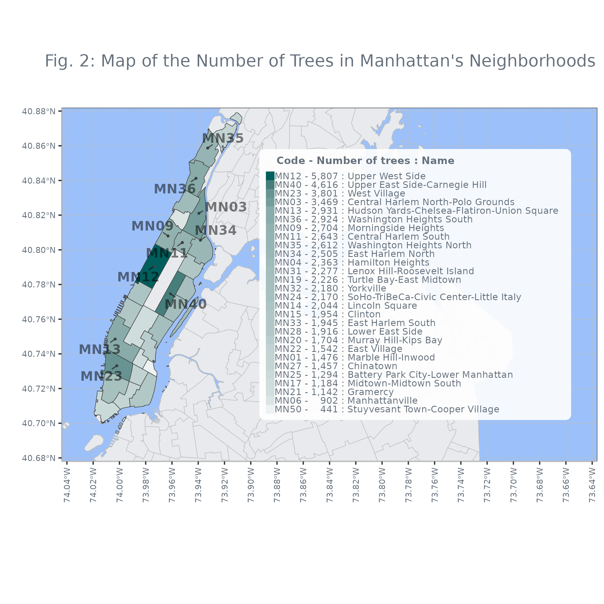
The top ten neighborhoods by tree counts are:
| Rank | NTA | NTA Name | Number of Trees | Percentage |
|---|---|---|---|---|
| 1 | MN12 | Upper West Side* | 5,807 | 9.04% |
| 2 | MN40 | Upper East Side–Carnegie Hill | 4,616 | 7.19% |
| 3 | MN23 | West Village* | 3,801 | 5.92% |
| 4 | MN03 | Central Harlem North–Polo Grounds* | 3,469 | 5.40% |
| 5 | MN13 | Hudson Yards–Chelsea–Flatiron–Union Square* | 2,931 | 4.56% |
| 6 | MN36 | Washington Heights South* | 2,924 | 4.55% |
| 7 | MN09 | Morningside Heights | 2,704 | 4.21% |
| 8 | MN11 | Central Harlem South | 2,643 | 4.11% |
| 9 | MN35 | Washington Heights North* | 2,612 | 4.07% |
| 10 | MN34 | East Harlem North* | 2,505 | 3.90% |
Seven of which (indicated by *) are part of the ten largest.
2.1.1.3. Trees by Curb Location
# Tree count per location in relation to curb
number_of_trees_per_curb_loc <- merged_trees_and_neighborhoods %>%
  filter(str_detect(nta, "MN") & !(nta == "MN99")) %>%
  group_by(curb_loc) %>%
  summarize(number_of_trees = n()) %>%
  arrange(desc(number_of_trees)) %>%
    mutate(percentage = label_percent(accuracy=0.01)(number_of_trees/length(merged_trees_and_neighborhoods$tree_id)))

on_curb_stat <- number_of_trees_per_curb_loc %>%
    mutate(proportion = number_of_trees/sum(number_of_trees)) %>%
  filter(proportion == max(abs(proportion)))

# Create a chart for curb location
curb_loc_stacked_bar_plot <- ggplot(number_of_trees_per_curb_loc) +
  geom_chicklet(aes(x="", y = number_of_trees/sum(number_of_trees),
                      fill = curb_loc),
                  radius = grid::unit(0.75, "mm"),
                  position="stack") +
  coord_flip() +
  theme(legend.position="right",
          legend.justification="top",
          legend.direction="vertical",
          legend.key.size = unit(0, 'pt'),
          #legend.key = element_rect(fill = NA),
          legend.text = element_text(margin = margin(r = 4, unit = "pt"),
                                     color = "#65707C",
                                     family="sans serif"),
          legend.title = element_text(color = "#65707C",
                                      face="bold",
                                      size = 9,
                                      family="sans serif"),
      axis.title.x = element_text(color="#65707C",
                                    face="bold",
                                    family="sans serif"),
      axis.title.y = element_blank(),
          axis.text = element_blank(),
          axis.line = element_blank(),
          axis.ticks = element_blank(),
          panel.grid.minor = element_blank(),
          panel.grid.major = element_blank(),
          panel.background = element_blank(),
      rect = element_rect(fill = "transparent"),
          plot.subtitle = element_text(color="#65707C",
                                    hjust=0.25,
                                    size=10,
                                    family="sans serif"),
          plot.title = element_text(color="#65707C",
                                    hjust=-0.15,
                                    size=14,
                                    family="sans serif"),
      plot.margin = unit(c(0,1,0,1), "cm")) +
  scale_fill_manual(values = c("#875826",
                                 "#10401B")) +
  ggtitle("\nFig. 3: Proportional Stacked Bar Graph of Tree Bed Location ",
            subtitle="  (in relation to the Curb)\n") +
  labs(y="\n%  \n(Number of trees)\n", fill="Location:  ") +
    guides(fill = guide_legend(nrow=2,
                               reverse=TRUE,
                               override.aes = list(shape = 15,
                                                   size = 4))) +
  scale_x_discrete(expand = c(0.01, 0)) +
  geom_text(data = on_curb_stat,
                             aes(label = paste(label_percent(accuracy=0.01)(proportion),
                                       "\n (", prettyNum(number_of_trees,
                                                  big.mark=","),")",
                                       sep=""),
                                 x = "",
                                 y = 0.50 * proportion - 0.075),
                            size=5, color="white", hjust=1)
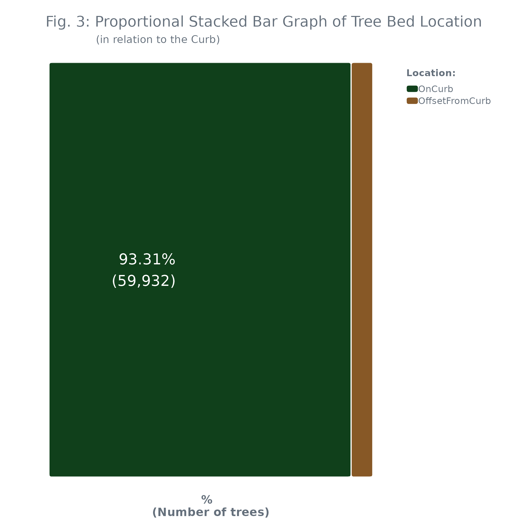
Majority or 93.31% (59,932) of the tree beds are located on curb, while the remaining 6.69% (4,297) are located offset from curb.
2.1.1.4. Tree Curb Location by Neigborhood
### Characteristics by Neighborhood

# Curb location per neighborhood
curb_loc_per_nbh <- merged_trees_and_neighborhoods %>%
	filter(str_detect(nta, "MN") & !(nta == "MN99")) %>%
	group_by(nta, nta_name, curb_loc) %>%
	summarize(number_of_trees=n(), .groups="keep") %>%
	group_by(nta) %>%
	mutate(proportion = number_of_trees/sum(number_of_trees),
           percentage = label_percent(accuracy=0.01)(proportion)) %>%
	arrange(desc(proportion)) %>%
	ungroup()

# Higher between OnCurb and OffsetFromCurb per neighborhood
oncurb_vs_offset_per_nbh <- curb_loc_per_nbh %>%
	group_by(nta) %>%
	filter(proportion == max(abs(proportion)))

# Order by NTA
curb_loc_per_nbh$nta_name <- factor(
    curb_loc_per_nbh$nta_name,
       levels = rev(unique(curb_loc_per_nbh$nta_name)),
       ordered=TRUE
)

# Table of Top 10 NTAs with the highest % of on-curb-located trees
top_on_curb <- curb_loc_per_nbh %>%
	filter(curb_loc=="OnCurb") %>%
	top_n(10, proportion) %>%
	arrange(desc(proportion)) %>%
    rownames_to_column("rank") %>%
	rename(number_of_on_curb_trees = number_of_trees)

# Table of Top 10 NTAs with the highest % of offset-from-curb-located trees
top_offset <- curb_loc_per_nbh %>%
	filter(curb_loc=="OffsetFromCurb") %>%
	top_n(10, proportion) %>%
	arrange(desc(proportion)) %>%
    rownames_to_column("rank") %>%
	rename(number_of_offset_from_curb_trees = number_of_trees)

# Proportional stacked bar graph of curb location per neighborhood
curb_loc_per_nbh_stacked_bar_plot <- ggplot(curb_loc_per_nbh) +
	geom_chicklet(aes(x = nta_name, y = proportion*100, fill = curb_loc),
                  radius = grid::unit(0.75, "mm"), position="stack") +
	coord_flip() +
	theme(legend.position="right",
          legend.justification="top",
          legend.direction="vertical",
          legend.key.size = unit(0, "pt"),
          legend.key = element_rect(fill=NA),
          legend.text = element_text(margin = margin(r = 4, unit = "pt"),
                                     color="#65707C",
                                     family="sans serif"),
          legend.title = element_text(color="#65707C",
                                      face="bold",
                                      size=9,
                                      family="sans serif"),
		  axis.title = element_text(color="#65707C",
                                    face="bold",
                                    family="sans serif"),
          axis.text.x = element_text(color="#65707C",
                                   size=6,
                                   family="sans serif"),
          axis.text.y = element_text(color="#65707C",
                                   size=10,
                                   family="sans serif"),
          axis.line = element_line(colour="grey",
                                   linewidth=0.5),
          panel.grid.major = element_line(color="grey",
                                          linetype="dashed",
                                          linewidth=0.25),
          panel.background = element_blank(),
          plot.subtitle = element_text(color="#65707C",
                                    hjust=5.38,
                                    size=10,
                                    family="sans serif"),
          plot.title = element_text(color = "#65707C",
                                    hjust = 0.709,
                                    size= 12.2,
                                    family = "sans serif")) +
	scale_fill_manual(values = c("#875826",
                                 "#10401B")) +
	ggtitle("\nFig. 4: Proportional Stacked Bar Graph of Each Neighborhood's Tree Bed Location",
            subtitle="               (in relation to the Curb)\n") +
	labs(x="\nNTA name \n", y="\nNTA code - % of on trees\n", fill="Location: ") +
    guides(fill = guide_legend(ncol=1,
                               reverse=TRUE,
                               override.aes = list(shape = 15,
                                                   size = 4))) +
	scale_y_continuous(expand = c(0.01, 0),
                       breaks = seq(0, 100, by=10)) +
	ggrepel::geom_text_repel(data = oncurb_vs_offset_per_nbh,
                             aes(label = paste(nta, " - ",
                                               label_percent(accuracy=0.01)(proportion),
                                       sep=""),
                                 x = nta_name,
                                 y = ifelse(nta=="MN50", 100*proportion+22,
                                            100*proportion-22)),
                             size=2.2, color="white", hjust=1)
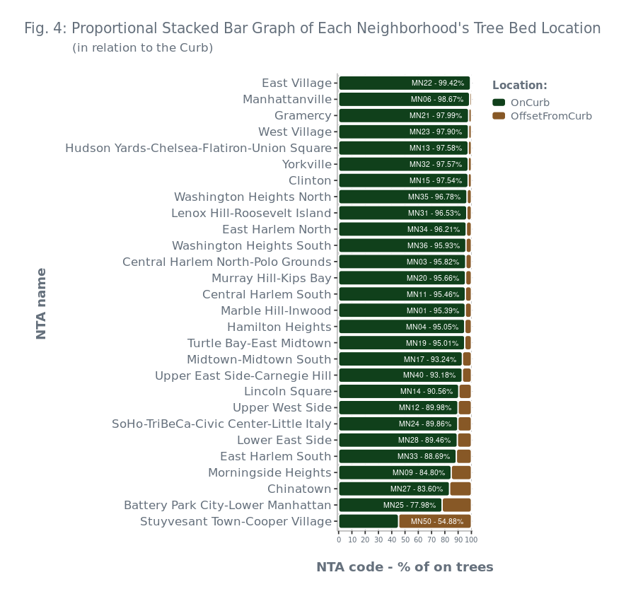
Twenty neighborhoods have at least 90% of their trees being on curb, while 27 have at least 75%. The ten neighborhoods with the highest percentage of trees located on-curb are:
| Rank | NTA | NTA Name | Number of On-Curb Trees | Percentage |
|---|---|---|---|---|
| 1 | MN22 | East Village | 1,533 | 99.42% |
| 2 | MN06 | Manhattanville | 890 | 98.67% |
| 3 | MN21 | Gramercy | 1,119 | 97.99% |
| 4 | MN23 | West Village | 3,721 | 97.90% |
| 5 | MN13 | Hudson Yards–Chelsea–Flatiron–Union Square | 2,860 | 97.58% |
| 6 | MN32 | Yorkville | 2,127 | 97.57% |
| 7 | MN15 | Clinton | 1,906 | 97.54% |
| 8 | MN35 | Washington Heights North | 2,528 | 96.78% |
| 9 | MN31 | Lenox Hill–Roosevelt Island | 2,198 | 96.53% |
| 10 | MN34 | East Harlem North | 2,410 | 96.21% |
Only Stuyvesant Town-Cooper Village has the majority of its trees being offset from curb. Including it, the neighborhoods with the highest percentage of trees located offset from curb are:
| Rank | NTA | NTA Name | Number of Offset-from-Curb Trees | Percentage |
|---|---|---|---|---|
| 1 | MN50 | Stuyvesant Town–Cooper Village | 242 | 54.88% |
| 2 | MN25 | Battery Park City–Lower Manhattan | 285 | 22.02% |
| 3 | MN27 | Chinatown | 239 | 16.40% |
| 4 | MN09 | Morningside Heights | 411 | 15.20% |
| 5 | MN33 | East Harlem South | 220 | 11.31% |
| 6 | MN28 | Lower East Side | 202 | 10.54% |
| 7 | MN24 | SoHo–TriBeCa–Civic Center–Little Italy | 220 | 10.14% |
| 8 | MN12 | Upper West Side | 582 | 10.02% |
| 9 | MN14 | Lincoln Square | 193 | 9.44% |
| 10 | MN40 | Upper East Side–Carnegie Hill | 315 | 6.82% |
2.1.2. Biological
2.1.2.1. Tree Size
# Species
nta_spc <- as.data.frame.matrix(table(trees$nta, trees$spc_common))

# Tree size (in terms of trunk diameter)
nta_tree_dbh <- as.data.frame.matrix(table(trees$nta, trees$tree_dbh)) %>%
  rename_with( ~ paste0(.x, "_tree_dbh"))

# Summary statistics of the trunk diameter
tree_dbh_stats <- data.frame(N = length(trees$tree_dbh),
                 mean = mean(trees$tree_dbh),
                             sd = sd(trees$tree_dbh),
                             min = min(trees$tree_dbh),
                             first_quartile = quantile(trees$tree_dbh, probs = 0.25),
                             median = median(trees$tree_dbh),
                             second_quartile = quantile(trees$tree_dbh, probs = 0.75),
                             max = max(trees$tree_dbh))
row.names(tree_dbh_stats) <- "tree_dbh"

# Density curve for 'tree_dbh'
tree_dbh_dist_plot <- ggplot(trees, aes(x = tree_dbh)) +
  geom_histogram(aes(y = after_stat(density)),
                   binwidth=1.1,
                   color=1,
                   fill="#5FBD5F") +
  geom_density(linewidth=0.85,
                 linetype=1,
                 colour = muted("5FBD5F"),
                 alpha=0.5) +

# Plot mean and median
geom_vline(aes(xintercept = mean(tree_dbh)), col="red", size=0.6) +
geom_vline(aes(xintercept = median(tree_dbh)), col="blue", size=0.6) +

     theme(axis.title = element_text(color="#65707C",
                                    face="bold",
                                    family="sans serif"),
          axis.text = element_text(color="#65707C",
                                   size=12,
                                   family="sans serif"),
          axis.line = element_line(colour="grey",
                                   linewidth=0.5),
          panel.grid.major = element_line(color="grey",
                                          linetype="dashed",
                                          linewidth=0.25),
          panel.background = element_blank(),
          plot.subtitle = element_text(color="#65707C",
                                    hjust=0.15,
                                    size=10,
                                    family="sans serif"),
          plot.title = element_text(color="#65707C",
                                    hjust=0.20,
                                    size=14,
                                    family="sans serif")) +
  ggtitle("\nFig. 5: Distribution of the Trunk Diameter") +
  labs(x="\nTrunk diameter in inches\n", y="\nDensity\n",
         subtitle="                (measured at 54 inches above the ground)\n") +
  scale_x_continuous(expand = c(0.01, 0),
                       limits = c(0, 105),
                       breaks = seq(0, 105, by=10)) +
  scale_y_continuous(expand = c(0.01, 0),
                       limits = c(0, 0.12),
                       breaks = seq(0, 0.12, by=0.02))
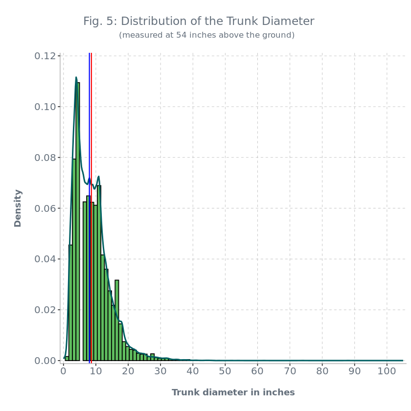
In terms of trunk diameter, the mean size of the tree population (red line in Fig. 5) is 8.6312 inches, with a standard deviation of 5.5906. Furthermore, its distribution is positively skewed, implying that the majority of trees have trunk diameters closer to the lower bound. In this case, we can use the median (blue line) of 8 inches (with an IQR of 7) as a better measure of central tendency (and spread).
2.1.2.2. Health-Related
# Status and health
pop_status <- as.data.frame(table(trees$status)) %>%
  mutate(attribute = "status", proportion = Freq/sum(Freq)) %>%
  rename(category = Var1, number_of_trees = Freq) %>%
  select(attribute, everything())

pop_health <- as.data.frame(table(trees$health)) %>%
  mutate(attribute = "health", proportion = Freq/sum(Freq)) %>%
  rename(category = Var1, number_of_trees = Freq) %>%
  select(attribute, everything()) %>%
  arrange(desc(proportion))

# Root problems
pop_root_stone <- as.data.frame(table(trees$root_stone)) %>%
  mutate(attribute = "root_stone", proportion = Freq/sum(Freq)) %>%
  rename(category = Var1, number_of_trees = Freq) %>%
  select(attribute, everything())

pop_root_grate <- as.data.frame(table(trees$root_grate)) %>%
  mutate(attribute = "root_grate", proportion = Freq/sum(Freq)) %>%
  rename(category = Var1, number_of_trees = Freq) %>%
  select(attribute, everything())

pop_root_other <- as.data.frame(table(trees$root_other)) %>%
  mutate(attribute = "root_other", proportion = Freq/sum(Freq)) %>%
  rename(category = Var1, number_of_trees = Freq) %>%
  select(attribute, everything())

# Trunk problems
pop_trunk_wire <- as.data.frame(table(trees$trunk_wire)) %>%
  mutate(attribute = "trunk_wire", proportion = Freq/sum(Freq)) %>%
  rename(category = Var1, number_of_trees = Freq) %>%
  select(attribute, everything())

pop_trnk_light <- as.data.frame(table(trees$trnk_light)) %>%
  mutate(attribute = "trnk_light", proportion = Freq/sum(Freq)) %>%
  rename(category = Var1, number_of_trees = Freq) %>%
  select(attribute, everything())

pop_trnk_other <- as.data.frame(table(trees$trnk_other)) %>%
  mutate(attribute = "trnk_other", proportion = Freq/sum(Freq)) %>%
  rename(category = Var1, number_of_trees = Freq) %>%
  select(attribute, everything())

# Branch problems
pop_brch_light <- as.data.frame(table(trees$brch_light)) %>%
  mutate(attribute = "brch_light", proportion = Freq/sum(Freq)) %>%
  rename(category = Var1, number_of_trees = Freq) %>%
  select(attribute, everything())

pop_brch_shoe <- as.data.frame(table(trees$brch_shoe)) %>%
  mutate(attribute = "brch_shoe", proportion = Freq/sum(Freq)) %>%
  rename(category = Var1, number_of_trees = Freq) %>%
  select(attribute, everything())

pop_brch_other <- as.data.frame(table(trees$brch_other)) %>%
  mutate(attribute = "brch_other", proportion = Freq/sum(Freq)) %>%
  rename(category = Var1, number_of_trees = Freq) %>%
  select(attribute, everything())

# Tree population's attributes
pop_attributes <- bind_rows(pop_status,
                            pop_health,
                            pop_root_stone,
                            pop_root_grate,
                            pop_root_other,
                            pop_trunk_wire,
                            pop_trnk_light,
                            pop_trnk_other,
                            pop_brch_light,
                            pop_brch_shoe,
                            pop_brch_other) %>%
                  mutate(percentage = label_percent(accuracy = 0.01)(proportion))

# Status and health
nta_status <- as.data.frame.matrix(table(trees$nta, trees$status)) %>%
  rename_with( ~ paste0(.x, "_status"))
nta_health <- as.data.frame.matrix(table(trees$nta, trees$health)) %>%
  rename_with( ~ paste0(.x, "_health"))

# Root problems
nta_root_stone <- as.data.frame.matrix(table(trees$nta, trees$root_stone)) %>%
  rename_with( ~ paste0(.x, "_root_stone"))
nta_root_grate <- as.data.frame.matrix(table(trees$nta, trees$root_grate)) %>%
  rename_with( ~ paste0(.x, "_root_grate"))
nta_root_other <- as.data.frame.matrix(table(trees$nta, trees$root_other)) %>%
  rename_with( ~ paste0(.x, "_root_other"))

# Trunk problems
nta_trunk_wire <- as.data.frame.matrix(table(trees$nta, trees$trunk_wire)) %>%
  rename_with( ~ paste0(.x, "_trunk_wire"))
nta_trnk_light <- as.data.frame.matrix(table(trees$nta, trees$trnk_light)) %>%
  rename_with( ~ paste0(.x, "_trnk_light"))
nta_trnk_other <- as.data.frame.matrix(table(trees$nta, trees$trnk_other)) %>%
  rename_with( ~ paste0(.x, "_trnk_other"))

# Branch problems
nta_brch_light <- as.data.frame.matrix(table(trees$nta, trees$brch_light)) %>%
  rename_with( ~ paste0(.x, "_brch_light"))
nta_brch_shoe <- as.data.frame.matrix(table(trees$nta, trees$brch_shoe)) %>%
  rename_with( ~ paste0(.x, "_brch_shoe"))
nta_brch_other <- as.data.frame.matrix(table(trees$nta, trees$brch_other)) %>%
  rename_with( ~ paste0(.x, "_brch_other"))

# Table of biological attributes per species
nta_bio <- bind_cols(list(nta_tree_dbh,
                          nta_status,
                          nta_health,
                          nta_root_stone,
                          nta_root_grate,
                          nta_root_other,
                          nta_trunk_wire,
                          nta_trnk_light,
                          nta_trnk_other,
                          nta_brch_light,
                          nta_brch_shoe,
                          nta_brch_other)) %>%
  rownames_to_column("nta")

# Highest category per attribute
pop_attributes_highest_per_category <- pop_attributes %>%
  group_by(attribute) %>%
  filter(proportion == max(abs(proportion)))

# Order by attributes
pop_attributes$attribute <- factor(
    pop_attributes$attribute,
       levels = rev(unique(pop_attributes$attribute)),
       ordered=TRUE
)

# Order by categories
pop_attributes$category <- factor(
    pop_attributes$category,
       levels = c("Dead", "Alive", "Fair", "Poor", "Good", "Yes", "No"),
       ordered=TRUE
)

pop_attributes_stacked_bar_plot <- ggplot(pop_attributes) +
  geom_chicklet(aes(x = attribute, y = proportion*100, fill = category),
                  radius = grid::unit(0.75, "mm"), position="stack") +
  coord_flip() +
  theme(legend.position = "right",
          legend.justification="top",
          legend.direction="vertical",
          legend.key.size = unit(0, "pt"),
          legend.key = element_rect(fill = NA),
          legend.text = element_text(margin = margin(r = 4, unit = "pt"),
                                     color = "#65707C",
                                     family="sans serif"),
          legend.title = element_text(color = "#65707C",
                                      face = "bold",
                                      size = 9,
                                      family="sans serif"),
      axis.title = element_text(color="#65707C",
                                    face="bold",
                                    family="sans serif"),
          axis.text = element_text(color="#65707C",
                                   size=12,
                                   family="sans serif"),
          axis.line = element_line(colour="grey",
                                   linewidth=0.5),
          panel.grid.major = element_line(color="grey",
                                          linetype="dashed",
                                          linewidth=0.25),
          panel.background = element_blank(),
          plot.title = element_text(color = "#65707C",
                                    hjust = 0.715,
                                    size= 13.75,
                                    family = "sans serif")) +
  scale_x_discrete(labels=c("Other problems (branch)",
                              "Shoes (branch)",
                              "Lights or wires (branch) ",
                              "Other problems (trunk)",
                              "Lighting installed (trunk)",
                              "Wires or rope (trunk)",
                              "Other problems (root)",
                              "Metal grates (root)",
                              "Paving stones (root)",
                              "Health",
                              "Status"))+
  scale_fill_manual(values = c("grey40",
                                 "#10401B",
                                 "#89E7B3",
                 "#40C17E",
                                 "#1F9153",
                                 "#9F2305",
                                 "#4E7A61"),
                     labels = c("Dead", "Alive", "Poor",  "Fair", "Good", "Yes", "No")) +
  ggtitle("\nFig. 6: Proportional Stacked Bar Graph of the Tree Population's Attributes\n") +
  labs(x="\nAttribute \n", y="\n%  \n(Number of trees) \n", fill="Category: ") +
    guides(fill = guide_legend(ncol=1,
                               override.aes = list(shape = 15,
                                                   size = 4))) +
  scale_y_continuous(expand = c(0.01, 0),
                       breaks = seq(0, 100, by=10)) +
  ggrepel::geom_text_repel(data = pop_attributes_highest_per_category,
                             aes(label = paste(percentage,
                                       "\n (", prettyNum(number_of_trees,
                                                  big.mark=","),")",
                                       sep=""),
                                 x = attribute,
                                 y = 100*proportion-20),
                             size=3, color="white", hjust=1)
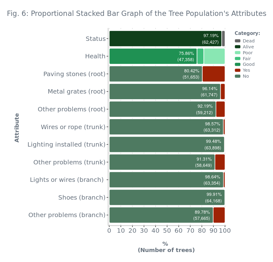
Nearly all of the trees in Manhattan have an “Alive” status, and majority are in a “Good” health condition. On the other hand, the minority of trees have problems with their roots, trunks, and branches. The most notable among these respective tree parts are caused by paving stones in the tree bed; trunk problems other than by wires/ropes and installed lighting; and branch problems other than by lights/wires and shoes.
2.2. Tree Species
Using spatial, descriptive, and correlation analyses, the following information outlines the biodiversity, biology, and ranking in terms of desirable traits of the tree species in Manhattan:
### Characteristics by Species

nbh_spc_long <- nta_spc %>%
  rownames_to_column("nta") %>%
  pivot_longer(cols = 2:129,
                 names_to = "spc_common",
                 values_to = "number_of_trees") %>%
  inner_join(trees %>% select(nta, nta_name) %>% distinct(nta, nta_name), by = "nta")

top_spc_per_nbh <- nbh_spc_long %>%
  group_by(nta) %>%
  top_n(1, number_of_trees) %>%
  arrange(nta, desc(number_of_trees)) %>%
  select(contains("nta"), everything()) %>%
  mutate(percentage = label_percent(accuracy=0.01)(
           number_of_trees/length(trees$tree_id)))

top_spc_per_nbh_short <- top_spc_per_nbh %>%
  group_by(spc_common) %>%
    mutate(nta = paste0(nta, collapse = ", "),
           nta_name = paste0(nta_name, collapse = ", ")) %>%
  count(nta, nta_name, spc_common) %>%
  arrange(desc(n)) %>%
    select(nta, nta_name, spc_common, n) %>%
  mutate(percentage = label_percent(accuracy=0.01)(n/28)) %>%
  rename(number_of_nta = n, most_common_spc = spc_common)

# Counts of neighborhood for the most common species
spc_in_top_ten_per_nbh <- nbh_spc_long %>%
  group_by(nta) %>%
  top_n(10, number_of_trees) %>%
  arrange(nta, desc(number_of_trees)) %>%
  select(contains("nta"), everything()) %>%
  ungroup() %>%
  count(spc_common) %>%
  mutate(percentage = label_percent(accuracy=0.01)(n/28)) %>%
  arrange(desc(n)) %>%
  rename(number_of_nta = n)

## Location

# Location in relation with the curb
spc_curb_loc <- as.data.frame.matrix(table(trees$spc_common, trees$curb_loc)) %>%
  rename_with( ~ paste0(.x, "_loc"))

## Biology

# Tree size (in terms of trunk diameter)
spc_tree_dbh <- as.data.frame.matrix(table(trees$spc_common, trees$tree_dbh)) %>%
  rename_with( ~ paste0(.x, "_tree_dbh"))

# Status and health
spc_status <- as.data.frame.matrix(table(trees$spc_common, trees$status)) #%>%
  #rename_with( ~ paste0(.x, "_status"))
spc_health <- as.data.frame.matrix(table(trees$spc_common, trees$health)) #%>%
  #rename_with( ~ paste0(.x, "_health"))

# Root problems
spc_root_stone <- as.data.frame.matrix(table(trees$spc_common, trees$root_stone)) %>%
  rename_with( ~ paste0(.x, "_root_stone"))
spc_root_grate <- as.data.frame.matrix(table(trees$spc_common, trees$root_grate)) %>%
  rename_with( ~ paste0(.x, "_root_grate"))
spc_root_other <- as.data.frame.matrix(table(trees$spc_common, trees$root_other)) %>%
  rename_with( ~ paste0(.x, "_root_other"))

# Trunk problems
spc_trunk_wire <- as.data.frame.matrix(table(trees$spc_common, trees$trunk_wire)) %>%
  rename_with( ~ paste0(.x, "_trunk_wire"))
spc_trnk_light <- as.data.frame.matrix(table(trees$spc_common, trees$trnk_light)) %>%
  rename_with( ~ paste0(.x, "_trnk_light"))
spc_trnk_other <- as.data.frame.matrix(table(trees$spc_common, trees$trnk_other)) %>%
  rename_with( ~ paste0(.x, "_trnk_other"))

# Branch problems
spc_brch_light <- as.data.frame.matrix(table(trees$spc_common, trees$brch_light)) %>%
  rename_with( ~ paste0(.x, "_brch_light"))
spc_brch_shoe <- as.data.frame.matrix(table(trees$spc_common, trees$brch_shoe)) %>%
  rename_with( ~ paste0(.x, "_brch_shoe"))
spc_brch_other <- as.data.frame.matrix(table(trees$spc_common, trees$brch_other)) %>%
  rename_with( ~ paste0(.x, "_brch_other"))

# Total number of identified species (Richness)
n_species <- trees %>%
  group_by(spc_common) %>%
  summarize(number_of_trees_per_species = n()) %>%
  filter(!is.na(spc_common)) %>%
  summarize(number_of_identified_species = n())

# Total number of trees with identified species (N_I) and unidentified species (N_U)
N_I_and_U <- trees %>%
  filter(is.na(spc_common)) %>%
  summarize(number_of_trees_with_unidentified_species = n()) %>%
  mutate(number_of_trees_with_identified_species = nrow(trees) - number_of_trees_with_unidentified_species)

# Top 10 NTAs with the highest species richness
top_ten_nbh_rchns <- nbh_rchns %>%
  slice(1:10) %>%
  rownames_to_column("rank")

# Order by richness
nbhs_map$nta_and_rchns <- factor(
    nbhs_map$nta_and_rchns,
       levels = (nbhs_map %>% arrange(desc(richness)))$nta_and_rchns,
       ordered = TRUE
)

# Map of NTAs' richness
nbh_rchns_map_plot <- ggplot() +
  geom_sf(data = nbhs_map %>% filter(borough != "MN" | nta == "MN99"),
            fill="#E8EAED", color="grey") +
  geom_sf(data = nbhs_map %>% filter(borough == "MN", nta != "MN99"),
            aes(fill = richness,
                color = nta_and_rchns
               )
           ) +
    stat_sf_coordinates(data = nbhs_map %>% filter(borough == "MN", nta != "MN99") %>%
                        inner_join(nbh_rchns, by = c("nta", "nta_name")) %>%
                          filter(nta %in% top_ten_nbh_rchns$nta),
                        color="grey25", size = 0.5) +
    theme(legend.position = c(0.3518, 0.5),
          legend.justification=0.0,
          legend.key.width = unit(2.5, 'mm'),
        legend.key.height = unit(1.8, 'mm'),
          legend.direction="vertical",
          legend.background = element_roundrect(r = grid::unit(0.02, "snpc"),
                                               fill = alpha("#FFFFFF", 0.90)),
          legend.key = element_rect(fill=NA),
          legend.text = element_text(margin = margin(r=5, unit="pt"),
                                   color="#65707C",
                                     family="sans serif"),
          legend.title = element_text(face="bold",
                                      color="#65707C",
                                      size=8.5,
                                      family="sans serif"),
          axis.title = element_text(color="#65707C",
                                    face="bold",
                                    family="sans serif"),
          axis.text = element_text(color="#65707C",
                                   size=7,
                                   family="sans serif"),
          axis.text.x = element_text(angle=90,
                                     vjust=0.5,
                                     hjust=1),
          axis.line = element_line(colour="grey",
                                   linewidth=0.5),
          panel.grid.major = element_line(color="grey",
                                          linetype="dashed",
                                          linewidth=0.25),

          panel.border = element_rect(color="grey40",
                                      fill=NA),
          panel.spacing = unit(2, "lines"),
          panel.background  = element_roundrect(r = grid::unit(0.001, "snpc"),
                                               fill = alpha("#9CC0F9", 1)),
          plot.title = element_text(color="#65707C",
                                    hjust=1.8,
                                    vjust=10,
                                    size=14,
                                    family="sans serif")) +
     labs(x="", y="", color="    Code - Richnesss : Name"
             ) +
     ggtitle("Fig. 7: Map of Tree Species Richness of Manhattan's Neighborhoods") +
  scale_x_continuous(expand = c(0.01, 0),
                       limits = c(-74.04, -73.64),
                       breaks = seq(-74.04, -73.64, by=0.02)) +
  scale_y_continuous(expand = c(0.01, 0),
                       limits = c(40.68, 40.88),
                       breaks = seq(40.68, 40.88, by=0.02)) +
  scale_color_manual(values = replicate(28, "grey25")) +
  scale_fill_gradient2(low = "#E3EDE5",
                         high = "#068409") +
  ggrepel::geom_label_repel(data = nbhs_map %>% filter(nta %in% top_ten_nbh_rchns$nta),
                              aes(label = nta, geometry = geometry),
                              stat="sf_coordinates",
                              min.segment.length=0,
                              label.size=NA,
                              alpha=0.5) +
  coord_sf(xlim = c(-74.04, -73.64), ylim = c(40.68, 40.88))

# Extract NTA fill colors
color_scheme_3 <- as.data.frame(ggplot_build(nbh_rchns_map_plot)$data[[2]])$fill

nbh_rchns_map_plot2 <- nbh_rchns_map_plot +
  guides(fill = "none",
           color = guide_legend(ncol=1,
                                override.aes = list(color = NA,
                                                    fill = color_scheme_3,
                                                    linewidth=0))
          )
2.2.1. Biodiversity
2.2.1.1. Richness
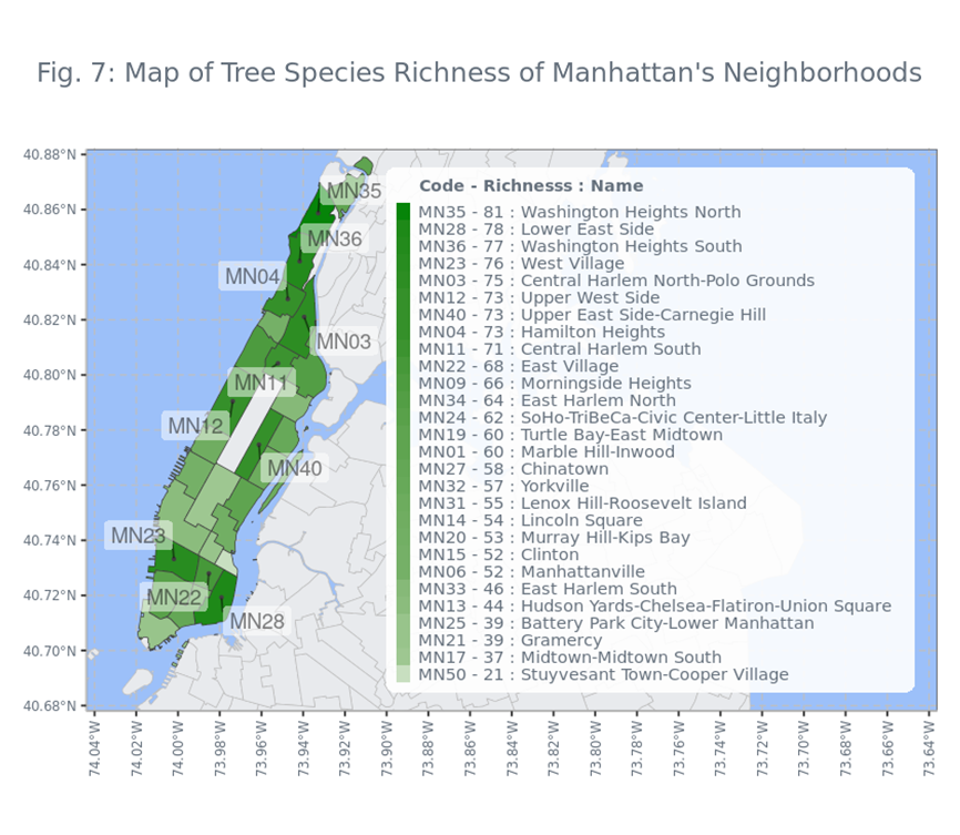
Richness is referred to as the number of species within a defined region. With respect to Manhattan, 128 species were identified among \({N_{I} =}\) 62,428 trees, while the remaining \({N_{U} =}\) 1,801 have species which are unidentified in the census. In terms of the neighborhoods, the ten with the highest richness (of identified species) are:
| Rank | NTA | NTA Name | Richness |
|---|---|---|---|
| 1 | MN35 | Washington Heights North | 81 |
| 2 | MN28 | Lower East Side | 78 |
| 3 | MN36 | Washington Heights South | 77 |
| 4 | MN23 | West Village | 76 |
| 5 | MN03 | Central Harlem North–Polo Grounds | 75 |
| 6 | MN04 | Hamilton Heights | 73 |
| 7 | MN12 | Upper West Side | 73 |
| 8 | MN40 | Upper East Side–Carnegie Hill | 73 |
| 9 | MN11 | Central Harlem South | 71 |
| 10 | MN22 | East Village | 68 |
2.2.1.2. Abundance
# Species abundance and relative abundance
spc_abd <- trees %>%
  filter(spc_common != "null") %>%
  group_by(spc_common) %>%
  summarize(abundance = n()) %>%
  ungroup() %>%
  mutate(relative_abundance = abundance/sum(abundance)) %>%
  arrange(desc(abundance))

# Species abundance and relative abundance by NTA
spc_abd_nbh <- nbh_spc_long %>%
  group_by(nta, nta_name) %>%
  filter(!(number_of_trees == 0)) %>%
  rename(abundance_wrt_nta = number_of_trees) %>%
  select(starts_with("nta"), spc_common, everything()) %>%
  mutate(relative_abundance_wrt_nta = label_percent(accuracy=0.01)(abundance_wrt_nta/sum(abundance_wrt_nta))) %>%
  arrange(nta, desc(abundance_wrt_nta)) %>%
  ungroup()

# Table for Top 10 Most Abundant Species
for_table_spc_abd <- spc_abd %>%
  slice(1:10) %>%
  rownames_to_column("rank") %>%
  mutate(abundance = prettyNum(abundance,big.mark=","),
           perc_relative_abundance = label_percent(accuracy=0.01)(relative_abundance))

# Bar graph for Top 25 tree species
top_species_bar_plot <- ggplot(spc_abd %>% slice(1:25)) +
  geom_chicklet(aes(x = fct_reorder(spc_common,
                                    abundance),
                      y = abundance),
                  fill="#10401B",
                  radius = grid::unit(1, "mm"), position="stack") +
  coord_flip() +
  theme(legend.position="none",
          axis.title = element_text(color = "#65707C",
                                    face="bold",
                                    family="sans serif"),
          axis.text = element_text(color = "#65707C",
                                   size=12,
                                   family="sans serif"),
          axis.title.x = element_text(margin=margin(20,0,10,0)),
          axis.title.y = element_text(margin=margin(0,20,0,10)),
          axis.line = element_line(colour = "grey",
                                   linewidth = 0.5),
          panel.grid.major = element_line(color = "grey",
                                          linetype="dashed",
                                          linewidth=0.25),
          panel.background = element_blank(),
          plot.title = element_text(color = "#65707C",
                                    hjust = 1.03,
                                    vjust = 4,
                                    size= 14,
                                    family = "sans serif",
                                    margin=margin(0,0,20,0))) +
  ggtitle("
\nFig. 8: Bar Graph of the 25 Most Abundant Tree Species in Manhattan ") +
  labs(x="Common name of the species", y="Abundance (% relative abundance)") +
  scale_y_continuous(expand = c(0.01, 0), limits = c(0,13500),
                      breaks = seq(0, 13500, by=2000)) +
  geom_text(aes(label = paste(prettyNum(abundance, big.mark=","),
                                " (", label_percent(accuracy=0.01)(relative_abundance),")",
                                sep=""),
                                 x = spc_common,
                                 y = ifelse(between(rank(desc(abundance)),3,10), abundance-807.5,
                                           ifelse(between(rank(desc(abundance)),2,2), abundance-880,
                                           ifelse(between(rank(desc(abundance)),1,1), abundance-980,
                                           ifelse(between(rank(desc(abundance)),11,11), abundance+770,
                                           abundance+670)))),
                  color = ifelse(between(rank(desc(abundance)),1,10), "white",
                                           "#65707C")),
              size = 2) +
scale_color_manual(values=c("#65707C","white"))
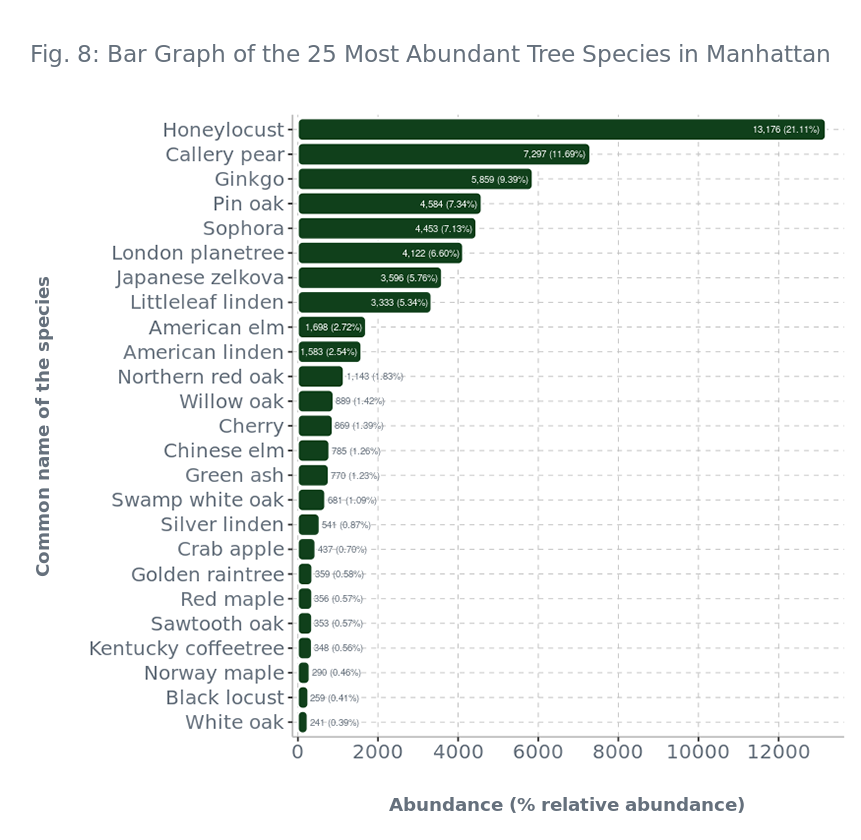
In this context, abundance is defined as the number of Manhattan trees per species, while relative abundance is the share of trees a certain species has in relation to the total number of trees in Manhattan. Among the 128 and other unidentified tree species in Manhattan, the ten most abundant are:
| Rank | Species (Common Name) | Abundance | Relative Abundance (%) |
|---|---|---|---|
| 1 | Honeylocust | 13,176 | 21.11% |
| 2 | Callery pear | 7,297 | 11.69% |
| 3 | Ginkgo | 5,859 | 9.39% |
| 4 | Pin oak | 4,584 | 7.34% |
| 5 | Sophora | 4,453 | 7.13% |
| 6 | London planetree | 4,122 | 6.60% |
| 7 | Japanese zelkova | 3,596 | 5.76% |
| 8 | Littleleaf linden | 3,333 | 5.34% |
| 9 | American elm | 1,698 | 2.72% |
| 10 | American linden | 1,583 | 2.54% |
2.2.1.3. Diversity
To describe the overall species diversity in Manhattan, a quantitative measure called Simpson’s Diversity Index (SDI) is used, which takes into account the species richness and evenness (or the distribution of abundance across the tree species in a community). The formula is given by:
where \({D} =\) Simpson’s Diversity Index (SDI);
\({n_{i} = i^{th}}\) species abundance;
\({N_{I} =}\) number of trees with identified species = 62,428
# Simpson's Diversity Index (SDI)
mnh_sdi <- spc_abd %>%
  filter(!is.na(spc_common)) %>%
   select(-relative_abundance) %>%
   mutate(numerator = abundance*(abundance-1)) %>%
   summarize(SDI = 1-(sum(numerator)/(sum(abundance)*(sum(abundance)-1))),
               number_of_trees = sum(abundance),
               richness = n())
With that, the computed SDI value is 0.909. This means that there is a very high diversity of tree species in Manhattan, and the chance of distinct species among two randomly selected trees from a sample is 90.9%.
2.2.2. Biology
2.2.2.1. Tree Size
# Summary statistics of species' tree dbh
spc_tree_dbh_stats <- trees %>%
  group_by(spc_common) %>%
  filter(!is.na(spc_common), !is.na(tree_dbh)) %>%
  summarize(abundance = n(),
              mean_tree_dbh = mean(tree_dbh),
              sd_tree_dbh = sd(tree_dbh),
              min_tree_dbh = min(tree_dbh),
              first_quartile_tree_dbh = quantile(tree_dbh, probs=0.25),
              median_tree_dbh = median(tree_dbh),
              third_quartile_tree_dbh = quantile(tree_dbh, probs=0.75),
              max_tree_dbh = max(tree_dbh))  %>%
  arrange(desc(median_tree_dbh))

# Top 25 species in terms of median dbh
top_spc_tree_dbh_stats <- spc_tree_dbh_stats #%>%
  #filter out species with abundances less than the median abundances
#filter(abundance >= median(abundance)) %>%
#select(spc_common, abundance, median_tree_dbh, everything())

# Bar graph for Top 30 tree species
top_spc_dbh_plot <- ggplot(top_spc_tree_dbh_stats %>% slice(1:25)) +
  geom_chicklet(aes(x = fct_reorder(spc_common,
                                    median_tree_dbh),
                      y = median_tree_dbh),
                  fill="#10401B",
                  radius = grid::unit(1, "mm"), position="stack") +
  coord_flip() +
  theme(axis.title = element_text(color = "#65707C",
                                    face="bold",
                                    family="sans serif"),
          axis.text = element_text(color = "#65707C",
                                   size=12,
                                   family="sans serif"),
          axis.title.x = element_text(margin=margin(20,0,10,0)),
          axis.title.y = element_text(margin=margin(0,20,0,10)),
          axis.line = element_line(colour = "grey",
                                   linewidth = 0.5),
          panel.grid.major = element_line(color = "grey",
                                          linetype="dashed",
                                          linewidth=0.25),
          panel.background = element_blank(),
          plot.title = element_text(color="#65707C",
                                    hjust=1.13,
                                    size=14,
                                    family="sans serif"),
          plot.subtitle = element_text(color="#65707C",
                                    hjust=2.02,
                                    size=10,
                                    family="sans serif")) +
  ggtitle("\nFig. 9: Bar Graph of the Top 25 Largest Tree Species in Manhattan",
            subtitle="(in terms of median trunk diameter at breast height (DBH) of 54 inches)\n") +
  labs(x="\nCommon name of the species\n", y="Trunk diameter in inches\n") +
  scale_y_continuous(expand = c(0.01, 0),
                       limits = c(0, 15.5),
                       breaks = seq(0, 15.5, by=3)) +
  geom_text(aes(label = median_tree_dbh,
                                 x = spc_common,
                                 y = median_tree_dbh-0.4),
              size = 3, color = "white")
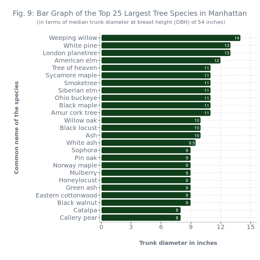
Tree sizes of the species were compared through their median trunk diameter at breast height (DBH). Fig. 9 shows the Top 25 largest species in terms of this metric:
2.2.2.2. Health-Related
# Status per species
spc_status <- trees %>%
  filter(!(is.na(spc_common) | is.na(spc_common))) %>%
  group_by(spc_common, status) %>%
  summarize(number_of_trees = n(), .groups="keep") %>%
  group_by(spc_common) %>%
  mutate(proportion_wrt_spc = number_of_trees/sum(number_of_trees),
           percentage_wrt_spc = label_percent(accuracy=0.01)(proportion_wrt_spc)) %>%
  arrange(proportion_wrt_spc) %>%
  select(-proportion_wrt_spc) %>%
  ungroup()
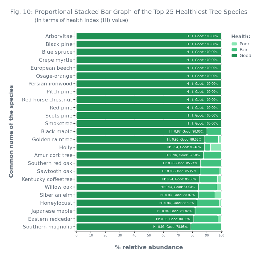
Out of the 128 species that have been identified, 127 have 100% of their trees being alive, while the remaining one, honeylocust, has 99.99%. As for the health, a numerical value called health index (\(HI\)) was computed for each species. This was done by assigning a number, \({j} ∈ \{1,2,3\}\), to the categories of Poor, Fair, and Good health, respectively, and then using the formula:
where \({HI_{i}} =\) health index of the \(i^{th}\) species;
\({a_{j}} =\) species abundance with respect to the \(j^{th}\) health category;
\({n_{i}} =\) \({i^{th}}\) species abundance
# Health per species
spc_health <- trees %>%
  filter(!is.na(spc_common), !is.na(health)) %>%
  group_by(spc_common, health) %>%
  summarize(number_of_trees = n(), .groups="keep") %>%
  group_by(spc_common) %>%
  mutate(proportion = number_of_trees/sum(number_of_trees),
           percentage = label_percent(accuracy=0.01)(proportion),
           health = as.factor(health)) %>%
  arrange(spc_common, desc(proportion)) %>%
  ungroup()

spc_health_index <- spc_health %>%
  group_by(spc_common) %>%
  mutate(health_score = ifelse(health=="Good", 3*number_of_trees,
                                 ifelse(health=="Fair", 2*number_of_trees,
                                        1*number_of_trees)),
          health_index = sum(health_score)/(3*sum(number_of_trees))) %>%
  ungroup() %>%
  select(spc_common, number_of_trees, health_index) %>%
  group_by(spc_common) %>%
  mutate(number_of_trees = sum(number_of_trees)) %>%
  distinct(spc_common, number_of_trees, health_index) %>%
  arrange(desc(health_index)) %>%
  ungroup() %>%
  rename(abundance = number_of_trees)

for_graph_top_spc_health <- spc_health %>%
  filter(spc_common %in% (
        spc_health_index %>%
        #filter out species with abundances less than the median abundances
#filter(abundance >= median(spc_tree_dbh_stats$abundance)) %>%
                              top_n(25, health_index))$spc_common) %>%
  arrange(desc(proportion))

# Order health per species
for_graph_top_spc_health$health <- factor(
    for_graph_top_spc_health$health,
    levels = c("Poor", "Fair", "Good"),
    ordered = TRUE
)

# Order species by proportion of 'Good' health
for_graph_top_spc_health$spc_common <- factor(
    for_graph_top_spc_health$spc_common,
    levels = rev((for_graph_top_spc_health %>% filter(health == "Good"))$spc_common),
    ordered = TRUE
)

top_spc_health_highest <- for_graph_top_spc_health %>%
  group_by(spc_common) %>%
  filter(proportion == max(abs(proportion)))

top_spc_health_stacked_bar_plot <- ggplot(for_graph_top_spc_health) +
  geom_chicklet(aes(x = spc_common, y = proportion*100, fill = health),
                  radius = grid::unit(0.75, "mm"), position="stack") +
  coord_flip() +
  theme(legend.position = "right",
          legend.justification="top",
          legend.direction="vertical",
          legend.key.size = unit(0, 'pt'),
          legend.key = element_rect(fill = NA),
          legend.text = element_text(margin = margin(r = 4, unit = "pt"),
                                     color = "#65707C",
                                     family="sans serif"),
          legend.title = element_text(color = "#65707C",
                                      face="bold",
                                      size = 9,
                                      family="sans serif"),
      axis.title = element_text(color="#65707C",
                                    face="bold",
                                    family="sans serif"),
          axis.text.x = element_text(color="#65707C",
                                   size=6,
                                   family="sans serif"),
          axis.text.y = element_text(color="#65707C",
                                   size=10,
                                   family="sans serif"),
          axis.line = element_line(colour="grey",
                                   linewidth=0.5),
          panel.grid.major = element_line(color="grey",
                                          linetype="dashed",
                                          linewidth=0.25),
          panel.background = element_blank(),
          plot.subtitle = element_text(color="#65707C",
                                    hjust=-2.07,
                                    size=10,
                                    family="sans serif"),
          plot.title = element_text(color = "#65707C",
                                    hjust = 0.74,
                                    size= 12,
                                    family = "sans serif")) +
  scale_fill_manual(values = c("#89E7B3",
                 "#40C17E",
                                 "#1F9153")) +
  ggtitle("\nFig. 10: Proportional Stacked Bar Graph of the Top 25 Healthiest Tree Species",
            subtitle="               (in terms of health index (HI) value)\n") +
  labs(x="\nCommon name of the species\n", y="\n% relative abundance\n", fill="Health: ") +
    guides(fill = guide_legend(ncol=1,
                               override.aes = list(shape = 15,
                                                   size = 4))) +
  scale_y_continuous(expand = c(0.01, 0),
                       breaks = seq(0, 100, by=10)) +
  ggrepel::geom_text_repel(data = top_spc_health_highest %>%
                              inner_join(spc_health_index, by="spc_common"),
                             aes(label = paste("HI: ", round(health_index, digits=2),
                                               ", Good: ", label_percent(
                                                   accuracy=0.01)(proportion), sep=""),
                                 x = spc_common,
                                 y = ifelse(proportion==1, 100*proportion-21.5,
                                            100*proportion-22)),
                             size=2.2, color="white", hjust=1)
Fig. 10 shows the 25 species with the highest HI value as well as the distribution of their relative abundances across health categories.
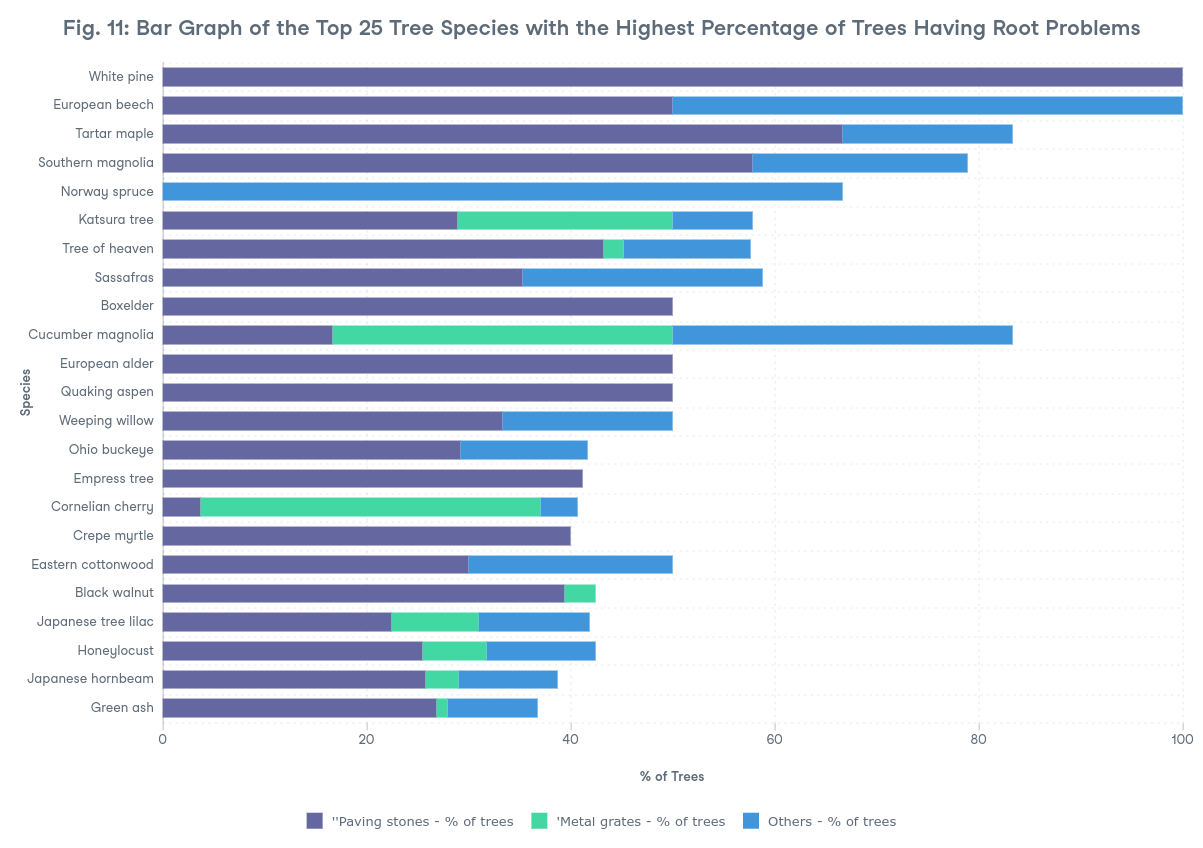
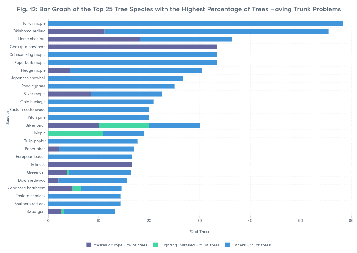
Paving stones as well as other trunk and branch problems also affect major tree parts (root, trunk, and branch) the most at a species level, similar to what is observed in the analysis of tree population.
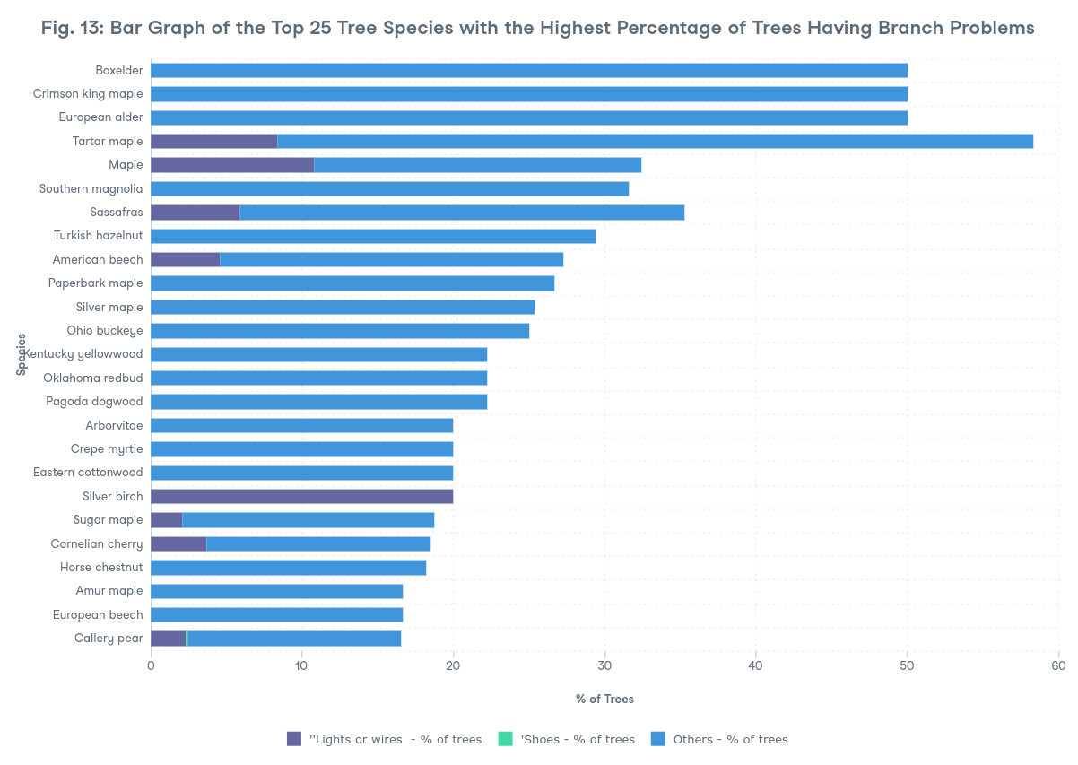
Figs. 11 to 13 show the top 25 species with the highest percentage of their trees having at least one problem for each tree part.
# For root problems' graph
spc_root_problems <- trees %>%
  select(spc_common, root_stone:root_other) %>%
  filter(spc_common != "null",
           if_all(-spc_common, ~ .x != "null")) %>%
  mutate(across(root_stone:root_other, ~ ifelse(.x == "Yes", 1, 0)),
           None = ifelse(root_stone == 0 &
                         root_grate == 0 &
                         root_other == 0, 1, 0)) %>%
  group_by(spc_common) %>%
  summarize(none = 100*sum(None)/n(),
              root_stone = 100*sum(root_stone)/n(),
              root_grate = 100*sum(root_grate)/n(),
              root_other = 100*sum(root_other)/n()) %>%
  rename(`Common name of the species` = spc_common,
           `''Paving stones` = root_stone,
           `'Metal grates` = root_grate,
           `Others` = root_other) %>%
  ungroup() %>%
  filter(rank((none)) <= 25) %>%
  arrange((none)) %>%
    mutate_if(is.numeric, ~(round(., digits = 2))) %>%
  pivot_longer(cols = c(3:5),
                 names_to = "Root problem",
                 values_to = "% of trees")
# For trunk problems' graph
spc_trunk_problems <- trees %>%
  select(spc_common, trunk_wire:trnk_other) %>%
  filter(spc_common != "null",
           if_all(-spc_common, ~ .x != "null")) %>%
  mutate(across(trunk_wire:trnk_other, ~ ifelse(.x == "Yes", 1, 0)),
           None = ifelse(trunk_wire == 0 &
                         trnk_light == 0 &
                         trnk_other == 0, 1, 0)) %>%
  group_by(spc_common) %>%
  summarize(none = 100*sum(None)/n(),
              trunk_wire = 100*sum(trunk_wire)/n(),
              trnk_light = 100*sum(trnk_light)/n(),
              trnk_other = 100*sum(trnk_other)/n()) %>%
  rename(`Common name of the species` = spc_common,
           `''Wires or rope` = trunk_wire,
           `'Lighting installed` = trnk_light,
           `Others` = trnk_other) %>%
  ungroup() %>%
  filter(rank((none)) <= 25) %>%
  arrange((none)) %>%
    mutate_if(is.numeric, ~(round(., digits = 2))) %>%
  pivot_longer(cols = c(3:5),
                 names_to = "Trunk problem",
                 values_to = "% of trees")
# For branch problems' graph
brch_trunk_problems <- trees %>%
  select(spc_common, brch_light:brch_other) %>%
  filter(spc_common != "null",
           if_all(-spc_common, ~ .x != "null")) %>%
  mutate(across(brch_light:brch_other, ~ ifelse(.x == "Yes", 1, 0)),
           None = ifelse(brch_light == 0 &
                         brch_shoe == 0 &
                         brch_other == 0, 1, 0)) %>%
  group_by(spc_common) %>%
  summarize(none = 100*sum(None)/n(),
              brch_light = 100*sum(brch_light)/n(),
              brch_shoe = 100*sum(brch_shoe)/n(),
              brch_other = 100*sum(brch_other)/n()) %>%
  rename(`Common name of the species` = spc_common,
           `''Lights or wires ` = brch_light,
           `'Shoes` = brch_shoe,
           `Others` = brch_other) %>%
  ungroup() %>%
  filter(rank((none)) <= 25) %>%
  arrange((none)) %>%
    mutate_if(is.numeric, ~(round(., digits = 2))) %>%
  pivot_longer(cols = c(3:5),
                 names_to = "Branch problem",
                 values_to = "% of trees")
2.2.3. Ranking
As suggested by the urban design team, tree size and health are used to determine which species have the most desirable characteristics. The two metrics used are health index (HI) and median trunk diameter at breast height (DBH) of 54 inches, respectively.
spearman_corr <- data.frame(
    test_stat=cor.test(spc_health_index$health_index, spc_tree_dbh_stats$median_tree_dbh,
         method = "spearman", exact = FALSE)$statistic,
    corr_coeff=cor.test(spc_health_index$health_index, spc_tree_dbh_stats$median_tree_dbh,
         method = "spearman", exact = FALSE)$estimate,
    p_value=cor.test(spc_health_index$health_index, spc_tree_dbh_stats$median_tree_dbh,
         method = "spearman", exact = FALSE)$p.value)

kendall_corr <- data.frame(
    test_stat=cor.test(spc_health_index$health_index, spc_tree_dbh_stats$median_tree_dbh,
         method = "kendall", exact = FALSE)$statistic,
    corr_coeff=cor.test(spc_health_index$health_index, spc_tree_dbh_stats$median_tree_dbh,
         method = "kendall", exact = FALSE)$estimate,
    p_value=cor.test(spc_health_index$health_index, spc_tree_dbh_stats$median_tree_dbh,
         method = "kendall", exact = FALSE)$p.value)

pearson_corr <- data.frame(
    test_stat=cor.test(spc_health_index$health_index, spc_tree_dbh_stats$median_tree_dbh)$statistic,
    corr_coeff=cor.test(spc_health_index$health_index, spc_tree_dbh_stats$median_tree_dbh)$estimate,
    p_value=cor.test(spc_health_index$health_index, spc_tree_dbh_stats$median_tree_dbh)$p.value)

corr_coeffs <- spearman_corr %>%
    mutate(method = "Spearman") %>%
  bind_rows(kendall_corr %>%
                mutate(method = "Kendall"),
              pearson_corr %>%
                mutate(method = "Pearson")) %>%
  select(method, everything()) %>%
  mutate(p_value = formatC(p_value, format = "e", digits = 4))

rownames(corr_coeffs) <- 1:nrow(corr_coeffs)

corr_coeffs %>%
  mutate_if(is.numeric, list(~round(., digits=4))) %>%
  mutate_if(is.numeric, list(~prettyNum(., big.mark=",")))
With that, it is confirmed through a correlation analysis that they have a high to very high positive correlation. This means that an increase in median trunk diameter is associated to an increase in the health index of a species. Below are the results of the correlation tests using three methods:
| Method | Test Statistic | Correlation Coefficient | p-value |
|---|---|---|---|
| Spearman | 4,759.501 | 0.9864 | 1.2123e-100 |
| Kendall | 14.7812 | 0.9361 | 1.9379e-49 |
| Pearson | 15.4671 | 0.8093 | 6.6475e-31 |
To determine species ranking, the sum of ranks for health index and median trunk diameter was computed to quantify each species’ overall rank relative to others.
Additionally, two ranking systems were produced. The first encompassed all 128 species. The second, however, adjusted for abundance by including only species with tree counts of at least 29, representing the median species abundance.
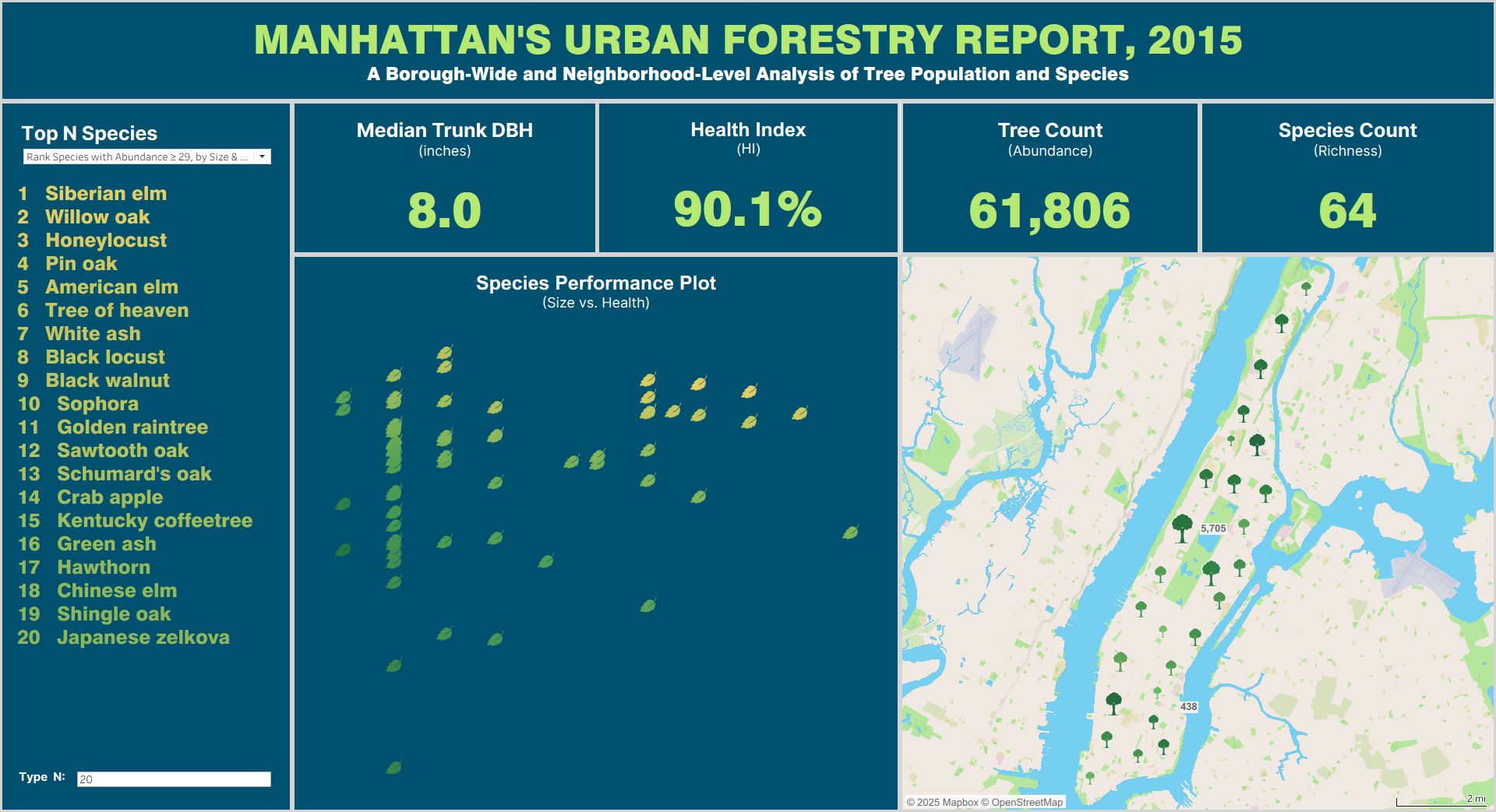
Figures 14 and 15 provide dashboard snapshots illustrating the results from both ranking systems.
# First Ranking System
spc_first_ranking <- spc_health_index %>%
  select(spc_common, abundance, health_index) %>%
  inner_join(trees %>%
               group_by(spc_common) %>%
               filter(spc_common != "null", health != "null") %>%
               summarize(abundance = n(),
                         median_tree_dbh = median(tree_dbh)),
      by=c("spc_common", "abundance")) %>%
  mutate(abd_rank = rank(desc(abundance)),
       hi_rank = rank(desc(health_index)),
       dbh_rank = rank(desc(median_tree_dbh)),
       rank_sum = (hi_rank + dbh_rank)/2) %>%
  arrange(rank_sum)

# Second Ranking System
spc_second_ranking <- spc_health_index %>%
  select(spc_common, abundance, health_index) %>%
  inner_join(trees %>%
               group_by(spc_common) %>%
               filter(spc_common != "null", health != "null") %>%
               summarize(abundance = n(),
                         median_tree_dbh = median(tree_dbh)),
      by=c("spc_common", "abundance")) %>%

# Filter out species with abundances less than the median abundances
  filter(abundance >= median(spc_tree_dbh_stats$abundance)
          ) %>%
mutate(abd_rank = rank(desc(abundance)),
       hi_rank = rank(desc(health_index)),
          dbh_rank = rank(desc(median_tree_dbh)),
       rank_sum = (hi_rank + dbh_rank)) %>%
  arrange(rank_sum)

# For graphs
spc_first_ranking_long <- spc_first_ranking %>%
  rename(`Common name of the species` = spc_common,
           `Health index` = health_index,
           `Median trunk dbh` = median_tree_dbh) %>%
  pivot_longer(cols = c(3:4),
                 names_to = "Measurement",
                 values_to = "Value")

spc_second_ranking_long <- spc_second_ranking %>%
  rename(`Common name of the species` = spc_common,
           `Health index` = health_index,
           `Median trunk dbh` = median_tree_dbh) %>%
  pivot_longer(cols = c(3:4),
                 names_to = "Measurement",
                 values_to = "Value")

# Tree size and Health
top_spc_first_ranking <- spc_first_ranking_long %>%
  arrange(rank_sum) %>%
  filter(`Common name of the species` %in% (spc_first_ranking %>% slice(1:10))$spc_common)

top_spc_second_ranking <- spc_second_ranking_long %>%
  arrange(rank_sum) %>%
  filter(`Common name of the species` %in% (spc_second_ranking %>% slice(1:10))$spc_common)


# Tree size
top_dbh_spc <- spc_second_ranking_long %>%
  arrange(desc(Measurement)) %>%
  filter(Measurement == "Median trunk dbh",
           `Common name of the species` %in% (spc_second_ranking %>% slice(1:10))$spc_common)

# Health
top_hi_spc <- spc_second_ranking_long %>%
  arrange(desc(Measurement)) %>%
  rename(`Health index` = Value) %>%
  filter(`Measurement` == "Health index",
           `Common name of the species` %in% (spc_second_ranking %>% slice(1:10))$spc_common)
Fig. 14: Dashboard Results Using ‘Rank All Species, by Size & Health’ System
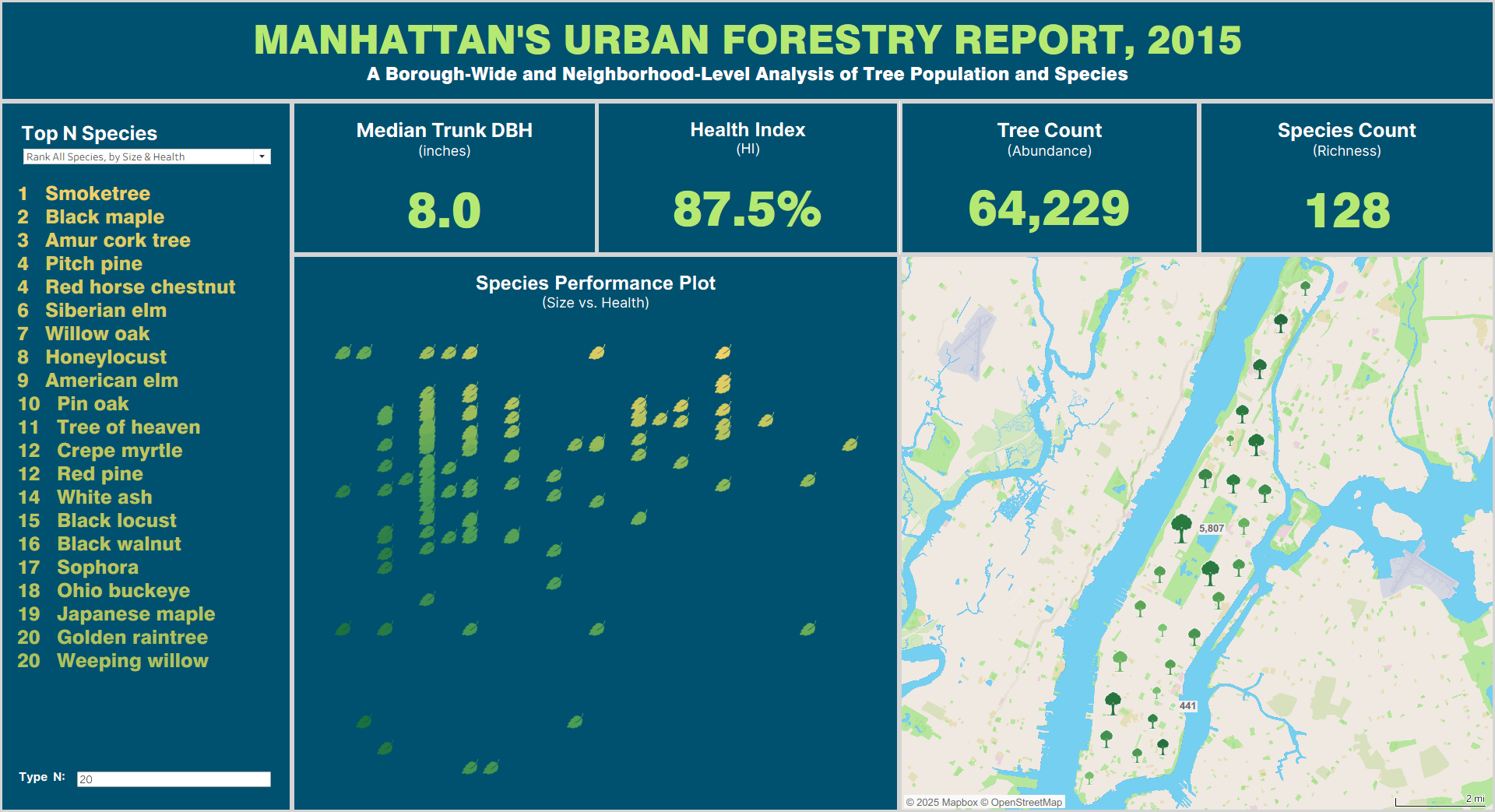
Fig. 15: Dashboard Results Using ‘Rank Species with Abundance ≥ 29, by Size & Health’
3. Recommendations
The following are some potential courses of action for Manhattan’s urban planning department:
Large southern neighborhoods such as Midtown-Midtown South (MN17), SoHo–TriBeCa–Civic Center–Little Italy (MN24), and Lower East Side (MN28), which are ranked third, sixth, and eighth in terms of land area, respectively, but only ranked 25th, 15th, and 19th in terms of tree counts, can be ideal locations for planting trees.
Some of the issues that need to be prioritized in the Stuyvesant Town-Cooper Village neighborhood include low tree counts, species richness, and a high number of trees that are offset from curb.
Although two rankings were produced, the second one has a better rank estimation due to large sample size per species; thus, the top five species (out of the 64 included) in terms of size and health that are recommended to be planted on the streets of Manhattan are:
Siberian elm
- Abundance: 156
- Median trunk diameter: 11 (3rd)
- Heath index: 0.9316 (6th)
Willow oak
- Abundance: 889
- Median trunk diameter: 10 (6th)
- Heath index: 0.9366 (5th)
Honeylocust
- Abundance: 13,176
- Median trunk diameter: 9 (12th)
- Heath index: 0.9387 (4th)
American elm
- Abundance: 1,698
- Median trunk diameter: 12 (2nd)
- Heath index: 0.9185 (17th)
Pin oak
- Abundance: 4,584
- Median trunk diameter: 9 (12th)
- Heath index: 0.9282 (9th)
- Trees of species Smoketree, Black maple, Amur cork tree, Pitch pine, and Red horse chestnut from the first ranking can also be considered as they have shown superior sizes and health. However, it is also suggested looking into related literature and/or more adequate data about them.
4. Appendix
4.1. Tables & Figures
4.1.1. Shape area per neighborhood
neighborhoods %>%
  filter(boroname == "Manhattan", ntacode != "MN99") %>%
  arrange(desc(shape_area)) %>%
  st_drop_geometry() %>%
  select(-boroname)
| ntacode | ntaname | shape_area | |
|---|---|---|---|
| 1 | MN13 | Hudson Yards-Chelsea-Flatiron-Union Square | 37029727 |
| 2 | MN12 | Upper West Side | 34381053 |
| 3 | MN17 | Midtown-Midtown South | 30192057 |
| 4 | MN03 | Central Harlem North-Polo Grounds | 25403425 |
| 5 | MN23 | West Village | 25000526 |
| 6 | MN24 | SoHo-TriBeCa-Civic Center-Little Italy | 24859569 |
| 7 | MN34 | East Harlem North | 24495420 |
| 8 | MN28 | Lower East Side | 23297616 |
| 9 | MN36 | Washington Heights South | 23100223 |
| 10 | MN35 | Washington Heights North | 22662313 |
| 11 | MN31 | Lenox Hill-Roosevelt Island | 21501565 |
| 12 | MN09 | Morningside Heights | 20158317 |
| 13 | MN40 | Upper East Side-Carnegie Hill | 20065329 |
| 14 | MN25 | Battery Park City-Lower Manhattan | 19056256 |
| 15 | MN15 | Clinton | 18381380 |
| 16 | MN01 | Marble Hill-Inwood | 17725321 |
| 17 | MN19 | Turtle Bay-East Midtown | 17397872 |
| 18 | MN33 | East Harlem South | 16650738 |
| 19 | MN04 | Hamilton Heights | 16093788 |
| 20 | MN14 | Lincoln Square | 15805668 |
| 21 | MN27 | Chinatown | 14501953 |
| 22 | MN20 | Murray Hill-Kips Bay | 14465848 |
| 23 | MN11 | Central Harlem South | 14436192 |
| 24 | MN32 | Yorkville | 13594780 |
| 25 | MN22 | East Village | 10895491 |
| 26 | MN06 | Manhattanville | 10647078 |
| 27 | MN21 | Gramercy | 7531455 |
| 28 | MN50 | Stuyvesant Town-Cooper Village | 5575232 |
4.1.2. Tree count per neighborhood
# Tree count per neighborhood
nbh_tree_cnts %>%
  mutate(Percentage = label_percent(accuracy=0.01)(proportion)) %>%
  select(-proportion)
| nta | nta_name | number_of_trees | Percentage |
|---|---|---|---|
| MN12 | Upper West Side | 5807 | 9.04% |
| MN40 | Upper East Side-Carnegie Hill | 4616 | 7.19% |
| MN23 | West Village | 3801 | 5.92% |
| MN03 | Central Harlem North-Polo Grounds | 3469 | 5.40% |
| MN13 | Hudson Yards-Chelsea-Flatiron-Union Square | 2931 | 4.56% |
| MN36 | Washington Heights South | 2924 | 4.55% |
| MN09 | Morningside Heights | 2704 | 4.21% |
| MN11 | Central Harlem South | 2643 | 4.11% |
| MN35 | Washington Heights North | 2612 | 4.07% |
| MN34 | East Harlem North | 2505 | 3.90% |
| MN04 | Hamilton Heights | 2363 | 3.68% |
| MN31 | Lenox Hill-Roosevelt Island | 2277 | 3.55% |
| MN19 | Turtle Bay-East Midtown | 2226 | 3.47% |
| MN32 | Yorkville | 2180 | 3.39% |
| MN24 | SoHo-TriBeCa-Civic Center-Little Italy | 2170 | 3.38% |
| MN14 | Lincoln Square | 2044 | 3.18% |
| MN15 | Clinton | 1954 | 3.04% |
| MN33 | East Harlem South | 1945 | 3.03% |
| MN28 | Lower East Side | 1916 | 2.98% |
| MN20 | Murray Hill-Kips Bay | 1704 | 2.65% |
| MN22 | East Village | 1542 | 2.40% |
| MN01 | Marble Hill-Inwood | 1476 | 2.30% |
| MN27 | Chinatown | 1457 | 2.27% |
| MN25 | Battery Park City-Lower Manhattan | 1294 | 2.01% |
| MN17 | Midtown-Midtown South | 1184 | 1.84% |
| MN21 | Gramercy | 1142 | 1.78% |
| MN06 | Manhattanville | 902 | 1.40% |
| MN50 | Stuyvesant Town-Cooper Village | 441 | 0.69% |
4.1.3. Tree count per curb location
number_of_trees_per_curb_loc
| curb_loc | number_of_trees | percentage |
|---|---|---|
| OnCurb | 59932 | 93.07% |
| OffsetFromCurb | 4297 | 6.67% |
4.1.4. Curb location per neighborhood
# Curb location per neighborhood
curb_loc_per_nbh %>%
  arrange(desc(curb_loc), desc(proportion)) %>%
  select(-proportion)
| nta | nta_name | curb_loc | number_of_trees | percentage |
|---|---|---|---|---|
| MN22 | East Village | OnCurb | 1533 | 99.42% |
| MN06 | Manhattanville | OnCurb | 890 | 98.67% |
| MN21 | Gramercy | OnCurb | 1119 | 97.99% |
| MN23 | West Village | OnCurb | 3721 | 97.90% |
| MN13 | Hudson Yards-Chelsea-Flatiron-Union Square | OnCurb | 2860 | 97.58% |
| MN32 | Yorkville | OnCurb | 2127 | 97.57% |
| MN15 | Clinton | OnCurb | 1906 | 97.54% |
| MN35 | Washington Heights North | OnCurb | 2528 | 96.78% |
| MN31 | Lenox Hill-Roosevelt Island | OnCurb | 2198 | 96.53% |
| MN34 | East Harlem North | OnCurb | 2410 | 96.21% |
| MN36 | Washington Heights South | OnCurb | 2805 | 95.93% |
| MN03 | Central Harlem North-Polo Grounds | OnCurb | 3324 | 95.82% |
| MN20 | Murray Hill-Kips Bay | OnCurb | 1630 | 95.66% |
| MN11 | Central Harlem South | OnCurb | 2523 | 95.46% |
| MN01 | Marble Hill-Inwood | OnCurb | 1408 | 95.39% |
| MN04 | Hamilton Heights | OnCurb | 2246 | 95.05% |
| MN19 | Turtle Bay-East Midtown | OnCurb | 2115 | 95.01% |
| MN17 | Midtown-Midtown South | OnCurb | 1104 | 93.24% |
| MN40 | Upper East Side-Carnegie Hill | OnCurb | 4301 | 93.18% |
| MN14 | Lincoln Square | OnCurb | 1851 | 90.56% |
| MN12 | Upper West Side | OnCurb | 5225 | 89.98% |
| MN24 | SoHo-TriBeCa-Civic Center-Little Italy | OnCurb | 1950 | 89.86% |
| MN28 | Lower East Side | OnCurb | 1714 | 89.46% |
| MN33 | East Harlem South | OnCurb | 1725 | 88.69% |
| MN09 | Morningside Heights | OnCurb | 2293 | 84.80% |
| MN27 | Chinatown | OnCurb | 1218 | 83.60% |
| MN25 | Battery Park City-Lower Manhattan | OnCurb | 1009 | 77.98% |
| MN50 | Stuyvesant Town-Cooper Village | OnCurb | 199 | 45.12% |
| MN50 | Stuyvesant Town-Cooper Village | OffsetFromCurb | 242 | 54.88% |
| MN25 | Battery Park City-Lower Manhattan | OffsetFromCurb | 285 | 22.02% |
| MN27 | Chinatown | OffsetFromCurb | 239 | 16.40% |
| MN09 | Morningside Heights | OffsetFromCurb | 411 | 15.20% |
| MN33 | East Harlem South | OffsetFromCurb | 220 | 11.31% |
| MN28 | Lower East Side | OffsetFromCurb | 202 | 10.54% |
| MN24 | SoHo-TriBeCa-Civic Center-Little Italy | OffsetFromCurb | 220 | 10.14% |
| MN12 | Upper West Side | OffsetFromCurb | 582 | 10.02% |
| MN14 | Lincoln Square | OffsetFromCurb | 193 | 9.44% |
| MN40 | Upper East Side-Carnegie Hill | OffsetFromCurb | 315 | 6.82% |
| MN17 | Midtown-Midtown South | OffsetFromCurb | 80 | 6.76% |
| MN19 | Turtle Bay-East Midtown | OffsetFromCurb | 111 | 4.99% |
| MN04 | Hamilton Heights | OffsetFromCurb | 117 | 4.95% |
| MN01 | Marble Hill-Inwood | OffsetFromCurb | 68 | 4.61% |
| MN11 | Central Harlem South | OffsetFromCurb | 120 | 4.54% |
| MN20 | Murray Hill-Kips Bay | OffsetFromCurb | 74 | 4.34% |
| MN03 | Central Harlem North-Polo Grounds | OffsetFromCurb | 145 | 4.18% |
| MN36 | Washington Heights South | OffsetFromCurb | 119 | 4.07% |
| MN34 | East Harlem North | OffsetFromCurb | 95 | 3.79% |
| MN31 | Lenox Hill-Roosevelt Island | OffsetFromCurb | 79 | 3.47% |
| MN35 | Washington Heights North | OffsetFromCurb | 84 | 3.22% |
| MN15 | Clinton | OffsetFromCurb | 48 | 2.46% |
| MN32 | Yorkville | OffsetFromCurb | 53 | 2.43% |
| MN13 | Hudson Yards-Chelsea-Flatiron-Union Square | OffsetFromCurb | 71 | 2.42% |
| MN23 | West Village | OffsetFromCurb | 80 | 2.10% |
| MN21 | Gramercy | OffsetFromCurb | 23 | 2.01% |
| MN06 | Manhattanville | OffsetFromCurb | 12 | 1.33% |
| MN22 | East Village | OffsetFromCurb | 9 | 0.58% |
4.1.5. Tree population’s categorical, health-related attributes
# Tree population's attributes
pop_attributes %>%
  select(-proportion)
| attribute | category | number_of_trees | percentage |
|---|---|---|---|
| status | Alive | 62427 | 97.19% |
| status | Dead | 1802 | 2.81% |
| health | Good | 47358 | 75.86% |
| health | Fair | 11460 | 18.36% |
| health | Poor | 3609 | 5.78% |
| root_stone | No | 51653 | 80.42% |
| root_stone | Yes | 12576 | 19.58% |
| root_grate | No | 61747 | 96.14% |
| root_grate | Yes | 2482 | 3.86% |
| root_other | No | 59212 | 92.19% |
| root_other | Yes | 5017 | 7.81% |
| trunk_wire | No | 63312 | 98.57% |
| trunk_wire | Yes | 917 | 1.43% |
| trnk_light | No | 63898 | 99.48% |
| trnk_light | Yes | 331 | 0.52% |
| trnk_other | No | 58649 | 91.31% |
| trnk_other | Yes | 5580 | 8.69% |
| brch_light | No | 63354 | 98.64% |
| brch_light | Yes | 875 | 1.36% |
| brch_shoe | No | 64168 | 99.91% |
| brch_shoe | Yes | 61 | 0.09% |
| brch_other | No | 57665 | 89.78% |
| brch_other | Yes | 6564 | 10.22% |
4.1.3. Richness (number of tree species) per neighborhood
nbh_rchns
| nta | nta_name | richness |
|---|---|---|
| MN35 | Washington Heights North | 81 |
| MN28 | Lower East Side | 78 |
| MN36 | Washington Heights South | 77 |
| MN23 | West Village | 76 |
| MN03 | Central Harlem North-Polo Grounds | 75 |
| MN04 | Hamilton Heights | 73 |
| MN12 | Upper West Side | 73 |
| MN40 | Upper East Side-Carnegie Hill | 73 |
| MN11 | Central Harlem South | 71 |
| MN22 | East Village | 68 |
| MN09 | Morningside Heights | 66 |
| MN34 | East Harlem North | 64 |
| MN24 | SoHo-TriBeCa-Civic Center-Little Italy | 62 |
| MN01 | Marble Hill-Inwood | 60 |
| MN19 | Turtle Bay-East Midtown | 60 |
| MN27 | Chinatown | 58 |
| MN32 | Yorkville | 57 |
| MN31 | Lenox Hill-Roosevelt Island | 55 |
| MN14 | Lincoln Square | 54 |
| MN20 | Murray Hill-Kips Bay | 53 |
| MN06 | Manhattanville | 52 |
| MN15 | Clinton | 52 |
| MN33 | East Harlem South | 46 |
| MN13 | Hudson Yards-Chelsea-Flatiron-Union Square | 44 |
| MN21 | Gramercy | 39 |
| MN25 | Battery Park City-Lower Manhattan | 39 |
| MN17 | Midtown-Midtown South | 37 |
| MN50 | Stuyvesant Town-Cooper Village | 21 |
4.1.6. Summary statistics of species abundances (number of trees per species)
defaultW <- getOption("warn")
options(warn=-1)

tree_attributes <- trees %>%
  select(spc_common, tree_dbh:brch_other) %>%
  filter(!is.na(spc_common))

spc_common <- levels(factor(tree_attributes$spc_common))

tree_attributes$spc_common <- factor(tree_attributes$spc_common,
                               levels = spc_common)

# Identified species abundances
identified_spc_abd <- trees %>%
  filter(!is.na(spc_common)) %>%
  group_by(spc_common) %>%
  summarize(abundance = n())

# Summary statistics of species abundances
spc_abd_stats <- data.frame(number_of_identified_spc = length(identified_spc_abd$abundance),
                mean = mean(identified_spc_abd$abundance),
                            sd = sd(identified_spc_abd$abundance),
                            min = min(identified_spc_abd$abundance),
                            first_quartile = quantile(identified_spc_abd$abundance, probs = 0.25),
                            median = median(identified_spc_abd$abundance),
                            third_quartile = quantile(identified_spc_abd$abundance, probs = 0.75),
                            max = max(identified_spc_abd$abundance))
row.names(spc_abd_stats) <- "spc_abundance"

# HTML Table for Number of Trees per Species
#kable(tree_dbh_stats %>%
#	  	mutate_if(is.numeric, list(~format(round(., 4), nsmall = 4))),
#     "html", caption = "Table _: Summary statistics of the tree diameter")

# Histogram with density curve of the species abundances
tree_count_per_species_dist_plot <- ggplot(identified_spc_abd,
                                           aes(x = abundance)) +
  geom_histogram(aes(y = after_stat(density)),
                   binwidth=25,
                   color=1,
                   fill="#5FBD5F") + geom_density(linewidth=0.85,
                                                  linetype=1,
                                                  colour = muted("5FBD5F"),
                                                  alpha=0.5) +

# Plot mean and median
  geom_vline(aes(xintercept = mean(abundance)), col="red", size=0.6) +
  geom_vline(aes(xintercept = median(abundance)), col="blue", size=0.6) +

  theme(axis.title = element_text(color="#65707C",
                                    face="bold",
                                    family="sans serif"),
          axis.text = element_text(color="#65707C",
                                   size=12,
                                   family="sans serif"),
          axis.line = element_line(colour="grey",
                                   linewidth=0.5),
          panel.grid.major = element_line(color="grey",
                                          linetype="dashed",
                                          linewidth=0.25),
          panel.background = element_blank(),
          plot.subtitle = element_text(color="#65707C",
                                    hjust=-0.33,
                                    size=10,
                                    family="sans serif"),
          plot.title = element_text(color="#65707C",
                                    hjust=0.5,
                                    size=14,
                                    family="sans serif")) +
  ggtitle("\nFig. 16: Distribution of the Species Abundance                \n") +
  labs(x="\nSpecies abundance\n", y="\nDensity\n") +
  scale_x_continuous(expand = c(0.01, 0),
                       limits = c(0, 2550),
                       breaks = seq(0, 2550, by=250)) +
  scale_y_continuous(expand = c(0.01, 0),
                       limits = c(0, 0.0081),
                       breaks = seq(0, 0.0081, by=0.001))

spc_abd_stats

options(warn = defaultW)
| number_of_identified_spc | mean | sd | min | first_quartile | median | third_quartile | max | |
|---|---|---|---|---|---|---|---|---|
| spc_abundance | 128 | 487.7188 | 1597.828 | 1 | 8.75 | 28.5 | 167.75 | 13176 |
4.1.7. Summary statistics of species’ tree DBHs
# Summary statistics of species' tree dbhs
spc_tree_dbh_stats
| spc_common | abundance | mean_tree_dbh | sd_tree_dbh | min_tree_dbh | first_quartile_tree_dbh | median_tree_dbh | third_quartile_tree_dbh | max_tree_dbh |
|---|---|---|---|---|---|---|---|---|
| Weeping willow | 12 | 13.500000 | 7.317476 | 4 | 8.00 | 14.0 | 19.00 | 26 |
| London planetree | 4122 | 13.168607 | 7.340801 | 1 | 7.00 | 13.0 | 18.00 | 48 |
| White pine | 1 | 13.000000 | NA | 13 | 13.00 | 13.0 | 13.00 | 13 |
| American elm | 1698 | 13.899293 | 9.703312 | 1 | 6.00 | 12.0 | 19.00 | 62 |
| Amur cork tree | 8 | 9.625000 | 3.925648 | 3 | 8.50 | 11.0 | 12.25 | 13 |
| Black maple | 10 | 12.600000 | 8.408990 | 4 | 5.00 | 11.0 | 19.50 | 26 |
| Ohio buckeye | 24 | 11.958333 | 5.368824 | 3 | 9.50 | 11.0 | 15.25 | 24 |
| Siberian elm | 156 | 12.064103 | 7.545714 | 2 | 5.75 | 11.0 | 17.00 | 33 |
| Smoketree | 1 | 11.000000 | NA | 11 | 11.00 | 11.0 | 11.00 | 11 |
| Sycamore maple | 23 | 11.521739 | 6.280341 | 2 | 7.50 | 11.0 | 16.00 | 26 |
| Tree of heaven | 104 | 11.451923 | 6.584595 | 2 | 5.00 | 11.0 | 16.00 | 34 |
| Ash | 58 | 9.603448 | 2.943561 | 3 | 8.00 | 10.0 | 11.75 | 16 |
| Black locust | 259 | 9.768340 | 4.735689 | 2 | 5.00 | 10.0 | 13.00 | 21 |
| Willow oak | 889 | 10.811024 | 9.331016 | 1 | 5.00 | 10.0 | 14.00 | 199 |
| White ash | 50 | 9.800000 | 4.347178 | 3 | 6.00 | 9.5 | 13.00 | 18 |
| Black walnut | 33 | 9.636364 | 6.004260 | 2 | 4.00 | 9.0 | 13.00 | 26 |
| Eastern cottonwood | 10 | 10.800000 | 6.178817 | 3 | 7.25 | 9.0 | 11.75 | 22 |
| Green ash | 770 | 9.255844 | 4.371351 | 0 | 6.00 | 9.0 | 12.00 | 28 |
| Honeylocust | 13176 | 9.058060 | 3.997006 | 0 | 6.00 | 9.0 | 11.00 | 109 |
| Mulberry | 68 | 11.000000 | 7.732467 | 1 | 5.00 | 9.0 | 15.00 | 44 |
| Norway maple | 290 | 10.237931 | 5.801379 | 2 | 6.00 | 9.0 | 13.00 | 35 |
| Pin oak | 4584 | 10.068499 | 7.982340 | 1 | 5.00 | 9.0 | 13.00 | 318 |
| Sophora | 4453 | 9.225915 | 4.892435 | 1 | 5.00 | 9.0 | 13.00 | 38 |
| Callery pear | 7297 | 8.681376 | 4.717342 | 1 | 6.00 | 8.0 | 11.00 | 228 |
| Catalpa | 13 | 8.538462 | 4.370648 | 4 | 6.00 | 8.0 | 9.00 | 21 |
| Ginkgo | 5859 | 8.445981 | 4.159496 | 1 | 5.00 | 8.0 | 11.00 | 74 |
| Pignut hickory | 1 | 8.000000 | NA | 8 | 8.00 | 8.0 | 8.00 | 8 |
| Pitch pine | 5 | 7.400000 | 3.286335 | 4 | 4.00 | 8.0 | 10.00 | 11 |
| Red horse chestnut | 1 | 8.000000 | NA | 8 | 8.00 | 8.0 | 8.00 | 8 |
| American hophornbeam | 84 | 8.345238 | 4.956422 | 2 | 4.00 | 7.5 | 12.00 | 22 |
| ⋮ | ⋮ | ⋮ | ⋮ | ⋮ | ⋮ | ⋮ | ⋮ | ⋮ |
| Shingle oak | 205 | 5.853659 | 4.2780847 | 1 | 3.00 | 4.0 | 7.00 | 30 |
| Southern red oak | 7 | 7.142857 | 4.4880794 | 3 | 4.00 | 4.0 | 10.50 | 14 |
| Sweetgum | 227 | 4.991189 | 3.3761149 | 2 | 3.00 | 4.0 | 6.00 | 22 |
| Tulip-poplar | 34 | 4.235294 | 0.9553303 | 2 | 4.00 | 4.0 | 5.00 | 6 |
| Turkish hazelnut | 17 | 4.764706 | 2.9053703 | 2 | 3.00 | 4.0 | 5.00 | 11 |
| White oak | 241 | 5.240664 | 2.9069181 | 2 | 3.00 | 4.0 | 7.00 | 17 |
| American beech | 22 | 5.227273 | 3.8412773 | 1 | 3.00 | 3.5 | 7.50 | 16 |
| Blackgum | 9 | 3.555556 | 2.5549516 | 2 | 2.00 | 3.0 | 4.00 | 10 |
| Chinese fringetree | 9 | 3.555556 | 1.6666667 | 2 | 2.00 | 3.0 | 4.00 | 7 |
| Common hackberry | 170 | 4.323529 | 2.8484459 | 1 | 2.00 | 3.0 | 5.00 | 14 |
| Eastern hemlock | 7 | 3.571429 | 0.7867958 | 3 | 3.00 | 3.0 | 4.00 | 5 |
| Eastern redcedar | 42 | 3.476190 | 2.1096537 | 2 | 2.00 | 3.0 | 4.00 | 10 |
| Hardy rubber tree | 66 | 3.803030 | 2.2750804 | 2 | 2.00 | 3.0 | 5.00 | 14 |
| Horse chestnut | 11 | 3.090909 | 0.7006490 | 2 | 3.00 | 3.0 | 3.50 | 4 |
| Kentucky yellowwood | 18 | 4.666667 | 3.2358288 | 2 | 3.00 | 3.0 | 4.00 | 14 |
| Mimosa | 12 | 3.750000 | 2.5980762 | 1 | 2.00 | 3.0 | 4.25 | 11 |
| Norway spruce | 3 | 4.000000 | 2.6457513 | 2 | 2.50 | 3.0 | 5.00 | 7 |
| Pagoda dogwood | 18 | 4.888889 | 4.4442810 | 2 | 2.25 | 3.0 | 4.00 | 16 |
| Paperbark maple | 15 | 3.266667 | 1.7099151 | 1 | 2.00 | 3.0 | 4.00 | 8 |
| Sassafras | 17 | 5.470588 | 4.2296224 | 2 | 3.00 | 3.0 | 6.00 | 16 |
| Spruce | 1 | 3.000000 | NA | 3 | 3.00 | 3.0 | 3.00 | 3 |
| Swamp white oak | 681 | 4.027900 | 2.4723381 | 0 | 3.00 | 3.0 | 4.00 | 32 |
| Blue spruce | 4 | 4.250000 | 3.8622101 | 2 | 2.00 | 2.5 | 4.75 | 10 |
| Pond cypress | 12 | 2.666667 | 0.8876254 | 2 | 2.00 | 2.5 | 3.00 | 5 |
| Scots pine | 2 | 2.500000 | 0.7071068 | 2 | 2.25 | 2.5 | 2.75 | 3 |
| Arborvitae | 5 | 3.400000 | 3.1304952 | 2 | 2.00 | 2.0 | 2.00 | 9 |
| Douglas-fir | 2 | 2.000000 | 1.4142136 | 1 | 1.50 | 2.0 | 2.50 | 3 |
| Himalayan cedar | 6 | 2.333333 | 0.5163978 | 2 | 2.00 | 2.0 | 2.75 | 3 |
| Persian ironwood | 1 | 2.000000 | NA | 2 | 2.00 | 2.0 | 2.00 | 2 |
| Osage-orange | 1 | 0.000000 | NA | 0 | 0.00 | 0.0 | 0.00 | 0 |
4.1.8. Status per species
# Status per species
spc_status
| spc_common | status | number_of_trees | percentage_wrt_spc |
|---|---|---|---|
| Honeylocust | Dead | 1 | 0.01% |
| Honeylocust | Alive | 13175 | 99.99% |
| 'Schubert' chokecherry | Alive | 163 | 100.00% |
| American beech | Alive | 22 | 100.00% |
| American elm | Alive | 1698 | 100.00% |
| American hophornbeam | Alive | 84 | 100.00% |
| American hornbeam | Alive | 85 | 100.00% |
| American larch | Alive | 7 | 100.00% |
| American linden | Alive | 1583 | 100.00% |
| Amur cork tree | Alive | 8 | 100.00% |
| Amur maackia | Alive | 59 | 100.00% |
| Amur maple | Alive | 30 | 100.00% |
| Arborvitae | Alive | 5 | 100.00% |
| Ash | Alive | 58 | 100.00% |
| Atlantic white cedar | Alive | 12 | 100.00% |
| Bald cypress | Alive | 89 | 100.00% |
| Bigtooth aspen | Alive | 5 | 100.00% |
| Black cherry | Alive | 32 | 100.00% |
| Black locust | Alive | 259 | 100.00% |
| Black maple | Alive | 10 | 100.00% |
| Black oak | Alive | 192 | 100.00% |
| Black pine | Alive | 3 | 100.00% |
| Black walnut | Alive | 33 | 100.00% |
| Blackgum | Alive | 9 | 100.00% |
| Blue spruce | Alive | 4 | 100.00% |
| Boxelder | Alive | 2 | 100.00% |
| Bur oak | Alive | 36 | 100.00% |
| Callery pear | Alive | 7297 | 100.00% |
| Catalpa | Alive | 13 | 100.00% |
| Cherry | Alive | 869 | 100.00% |
| ⋮ | ⋮ | ⋮ | ⋮ |
| Sawtooth oak | Alive | 353 | 100.00% |
| Scarlet oak | Alive | 71 | 100.00% |
| Schumard's oak | Alive | 137 | 100.00% |
| Scots pine | Alive | 2 | 100.00% |
| Serviceberry | Alive | 38 | 100.00% |
| Shingle oak | Alive | 205 | 100.00% |
| Siberian elm | Alive | 156 | 100.00% |
| Silver birch | Alive | 10 | 100.00% |
| Silver linden | Alive | 541 | 100.00% |
| Silver maple | Alive | 71 | 100.00% |
| Smoketree | Alive | 1 | 100.00% |
| Sophora | Alive | 4453 | 100.00% |
| Southern magnolia | Alive | 19 | 100.00% |
| Southern red oak | Alive | 7 | 100.00% |
| Spruce | Alive | 1 | 100.00% |
| Sugar maple | Alive | 48 | 100.00% |
| Swamp white oak | Alive | 681 | 100.00% |
| Sweetgum | Alive | 227 | 100.00% |
| Sycamore maple | Alive | 23 | 100.00% |
| Tartar maple | Alive | 12 | 100.00% |
| Tree of heaven | Alive | 104 | 100.00% |
| Tulip-poplar | Alive | 34 | 100.00% |
| Turkish hazelnut | Alive | 17 | 100.00% |
| Two-winged silverbell | Alive | 8 | 100.00% |
| Virginia pine | Alive | 3 | 100.00% |
| Weeping willow | Alive | 12 | 100.00% |
| White ash | Alive | 50 | 100.00% |
| White oak | Alive | 241 | 100.00% |
| White pine | Alive | 1 | 100.00% |
| Willow oak | Alive | 889 | 100.00% |
4.1.9. Health per species
# Health per species
spc_health %>%
  select(-proportion)
| spc_common | health | number_of_trees | percentage |
|---|---|---|---|
| 'Schubert' chokecherry | Good | 111 | 68.10% |
| 'Schubert' chokecherry | Fair | 40 | 24.54% |
| 'Schubert' chokecherry | Poor | 12 | 7.36% |
| American beech | Good | 15 | 68.18% |
| American beech | Fair | 4 | 18.18% |
| American beech | Poor | 3 | 13.64% |
| American elm | Good | 1361 | 80.15% |
| American elm | Fair | 259 | 15.25% |
| American elm | Poor | 78 | 4.59% |
| American hophornbeam | Good | 64 | 76.19% |
| American hophornbeam | Fair | 12 | 14.29% |
| American hophornbeam | Poor | 8 | 9.52% |
| American hornbeam | Good | 67 | 78.82% |
| American hornbeam | Fair | 13 | 15.29% |
| American hornbeam | Poor | 5 | 5.88% |
| American larch | Fair | 3 | 42.86% |
| American larch | Good | 3 | 42.86% |
| American larch | Poor | 1 | 14.29% |
| American linden | Good | 1020 | 64.43% |
| American linden | Fair | 379 | 23.94% |
| American linden | Poor | 184 | 11.62% |
| Amur cork tree | Good | 7 | 87.50% |
| Amur cork tree | Fair | 1 | 12.50% |
| Amur maackia | Good | 46 | 77.97% |
| Amur maackia | Fair | 10 | 16.95% |
| Amur maackia | Poor | 3 | 5.08% |
| Amur maple | Good | 19 | 63.33% |
| Amur maple | Fair | 7 | 23.33% |
| Amur maple | Poor | 4 | 13.33% |
| Arborvitae | Good | 5 | 100.00% |
| ⋮ | ⋮ | ⋮ | ⋮ |
| Sycamore maple | Fair | 7 | 30.43% |
| Sycamore maple | Poor | 2 | 8.70% |
| Tartar maple | Good | 5 | 41.67% |
| Tartar maple | Fair | 4 | 33.33% |
| Tartar maple | Poor | 3 | 25.00% |
| Tree of heaven | Good | 82 | 78.85% |
| Tree of heaven | Fair | 17 | 16.35% |
| Tree of heaven | Poor | 5 | 4.81% |
| Tulip-poplar | Good | 17 | 50.00% |
| Tulip-poplar | Fair | 10 | 29.41% |
| Tulip-poplar | Poor | 7 | 20.59% |
| Turkish hazelnut | Fair | 9 | 52.94% |
| Turkish hazelnut | Good | 7 | 41.18% |
| Turkish hazelnut | Poor | 1 | 5.88% |
| Two-winged silverbell | Good | 5 | 62.50% |
| Two-winged silverbell | Fair | 3 | 37.50% |
| Virginia pine | Good | 2 | 66.67% |
| Virginia pine | Poor | 1 | 33.33% |
| Weeping willow | Good | 8 | 66.67% |
| Weeping willow | Fair | 4 | 33.33% |
| White ash | Good | 40 | 80.00% |
| White ash | Fair | 8 | 16.00% |
| White ash | Poor | 2 | 4.00% |
| White oak | Good | 162 | 67.22% |
| White oak | Fair | 56 | 23.24% |
| White oak | Poor | 23 | 9.54% |
| White pine | Fair | 1 | 100.00% |
| Willow oak | Good | 747 | 84.03% |
| Willow oak | Fair | 115 | 12.94% |
| Willow oak | Poor | 27 | 3.04% |
4.1.10. Health index per species
spc_health_index %>%
  select(-abundance)
| spc_common | health_index |
|---|---|
| Arborvitae | 1.0000000 |
| Black pine | 1.0000000 |
| Blue spruce | 1.0000000 |
| Crepe myrtle | 1.0000000 |
| European beech | 1.0000000 |
| Osage-orange | 1.0000000 |
| Persian ironwood | 1.0000000 |
| Pitch pine | 1.0000000 |
| Red horse chestnut | 1.0000000 |
| Red pine | 1.0000000 |
| Scots pine | 1.0000000 |
| Smoketree | 1.0000000 |
| Black maple | 0.9666667 |
| Amur cork tree | 0.9583333 |
| Golden raintree | 0.9554318 |
| Southern red oak | 0.9523810 |
| Sawtooth oak | 0.9471199 |
| Kentucky coffeetree | 0.9415709 |
| Japanese maple | 0.9393939 |
| Honeylocust | 0.9387223 |
| Willow oak | 0.9366329 |
| Holly | 0.9358974 |
| Siberian elm | 0.9316239 |
| Southern magnolia | 0.9298246 |
| Eastern redcedar | 0.9285714 |
| Hawthorn | 0.9284627 |
| Pin oak | 0.9282286 |
| Crab apple | 0.9260107 |
| Blackgum | 0.9259259 |
| Shingle oak | 0.9252033 |
| ⋮ | ⋮ |
| Bigtooth aspen | 0.8000000 |
| Eastern cottonwood | 0.8000000 |
| Japanese snowbell | 0.8000000 |
| Hedge maple | 0.7971014 |
| Sassafras | 0.7843137 |
| Turkish hazelnut | 0.7843137 |
| Silver maple | 0.7840376 |
| Katsura tree | 0.7807018 |
| Cucumber magnolia | 0.7777778 |
| Kentucky yellowwood | 0.7777778 |
| Norway spruce | 0.7777778 |
| Pine | 0.7777778 |
| Virginia pine | 0.7777778 |
| Tulip-poplar | 0.7647059 |
| American larch | 0.7619048 |
| Horse chestnut | 0.7575758 |
| Pagoda dogwood | 0.7407407 |
| Tartar maple | 0.7222222 |
| Maple | 0.7027027 |
| Cockspur hawthorn | 0.6666667 |
| Douglas-fir | 0.6666667 |
| Paperbark maple | 0.6666667 |
| Pignut hickory | 0.6666667 |
| Spruce | 0.6666667 |
| White pine | 0.6666667 |
| Crimson king maple | 0.5555556 |
| Pond cypress | 0.5555556 |
| Eastern hemlock | 0.5238095 |
| Boxelder | 0.5000000 |
| European alder | 0.5000000 |
4.1.11. Species’ distribution of root problems
trees %>%
  select(spc_common, root_stone:root_other) %>%
  filter(spc_common != "null",
           if_all(-spc_common, ~ .x != "null")) %>%
  mutate(across(root_stone:root_other, ~ ifelse(.x == "Yes", 1, 0)),
           no_problem = ifelse(root_stone == 0 &
                               root_grate == 0 &
                               root_other == 0, 1, 0)) %>%
  group_by(spc_common) %>%
  summarize(no_problem = 100*sum(no_problem)/n(),
              root_stone = 100*sum(root_stone)/n(),
              root_grate = 100*sum(root_grate)/n(),
              root_other = 100*sum(root_other)/n()) %>%
  arrange(no_problem) %>%
    mutate_if(is.numeric, ~(round(., digits = 2)))
| spc_common | no_problem | root_stone | root_grate | root_other |
|---|---|---|---|---|
| White pine | 0.00 | 100.00 | 0.00 | 0.00 |
| European beech | 16.67 | 50.00 | 0.00 | 50.00 |
| Tartar maple | 16.67 | 66.67 | 0.00 | 16.67 |
| Southern magnolia | 26.32 | 57.89 | 0.00 | 21.05 |
| Norway spruce | 33.33 | 0.00 | 0.00 | 66.67 |
| Katsura tree | 42.11 | 28.95 | 21.05 | 7.89 |
| Tree of heaven | 45.19 | 43.27 | 1.92 | 12.50 |
| Sassafras | 47.06 | 35.29 | 0.00 | 23.53 |
| Boxelder | 50.00 | 50.00 | 0.00 | 0.00 |
| Cucumber magnolia | 50.00 | 16.67 | 33.33 | 33.33 |
| European alder | 50.00 | 50.00 | 0.00 | 0.00 |
| Quaking aspen | 50.00 | 50.00 | 0.00 | 0.00 |
| Weeping willow | 50.00 | 33.33 | 0.00 | 16.67 |
| Ohio buckeye | 58.33 | 29.17 | 0.00 | 12.50 |
| Empress tree | 58.82 | 41.18 | 0.00 | 0.00 |
| Cornelian cherry | 59.26 | 3.70 | 33.33 | 3.70 |
| Crepe myrtle | 60.00 | 40.00 | 0.00 | 0.00 |
| Eastern cottonwood | 60.00 | 30.00 | 0.00 | 20.00 |
| Black walnut | 60.61 | 39.39 | 3.03 | 0.00 |
| Japanese tree lilac | 62.02 | 22.48 | 8.53 | 10.85 |
| Honeylocust | 62.15 | 25.50 | 6.28 | 10.66 |
| Japanese hornbeam | 64.52 | 25.81 | 3.23 | 9.68 |
| Green ash | 65.45 | 26.88 | 1.04 | 8.83 |
| Cockspur hawthorn | 66.67 | 33.33 | 0.00 | 33.33 |
| Crimson king maple | 66.67 | 33.33 | 0.00 | 16.67 |
| Oklahoma redbud | 66.67 | 33.33 | 0.00 | 0.00 |
| Paperbark maple | 66.67 | 13.33 | 6.67 | 20.00 |
| Virginia pine | 66.67 | 33.33 | 0.00 | 0.00 |
| Norway maple | 67.24 | 27.93 | 1.03 | 7.93 |
| Callery pear | 67.60 | 20.87 | 7.02 | 8.17 |
| ⋮ | ⋮ | ⋮ | ⋮ | ⋮ |
| Eastern redbud | 92.00 | 4.00 | 0 | 4.00 |
| River birch | 92.59 | 3.70 | 0 | 3.70 |
| Magnolia | 93.10 | 5.17 | 0 | 1.72 |
| Bur oak | 94.44 | 2.78 | 0 | 2.78 |
| American hornbeam | 95.29 | 3.53 | 0 | 1.18 |
| Crab apple | 96.34 | 2.75 | 0 | 1.14 |
| Eastern redcedar | 97.62 | 0.00 | 0 | 2.38 |
| Hawthorn | 97.72 | 0.91 | 0 | 1.37 |
| European hornbeam | 98.20 | 0.00 | 0 | 1.80 |
| American larch | 100.00 | 0.00 | 0 | 0.00 |
| Arborvitae | 100.00 | 0.00 | 0 | 0.00 |
| Bigtooth aspen | 100.00 | 0.00 | 0 | 0.00 |
| Black pine | 100.00 | 0.00 | 0 | 0.00 |
| Blue spruce | 100.00 | 0.00 | 0 | 0.00 |
| Douglas-fir | 100.00 | 0.00 | 0 | 0.00 |
| Himalayan cedar | 100.00 | 0.00 | 0 | 0.00 |
| Kousa dogwood | 100.00 | 0.00 | 0 | 0.00 |
| Osage-orange | 100.00 | 0.00 | 0 | 0.00 |
| Persian ironwood | 100.00 | 0.00 | 0 | 0.00 |
| Pignut hickory | 100.00 | 0.00 | 0 | 0.00 |
| Pine | 100.00 | 0.00 | 0 | 0.00 |
| Pitch pine | 100.00 | 0.00 | 0 | 0.00 |
| Pond cypress | 100.00 | 0.00 | 0 | 0.00 |
| Red horse chestnut | 100.00 | 0.00 | 0 | 0.00 |
| Red pine | 100.00 | 0.00 | 0 | 0.00 |
| Scots pine | 100.00 | 0.00 | 0 | 0.00 |
| Smoketree | 100.00 | 0.00 | 0 | 0.00 |
| Southern red oak | 100.00 | 0.00 | 0 | 0.00 |
| Spruce | 100.00 | 0.00 | 0 | 0.00 |
| Two-winged silverbell | 100.00 | 0.00 | 0 | 0.00 |
4.1.12. Species’ distribution of trunk problems
trees %>%
  select(spc_common, trunk_wire:trnk_other) %>%
  filter(spc_common != "null",
           if_all(-spc_common, ~ .x != "null")) %>%
  mutate(across(trunk_wire:trnk_other, ~ ifelse(.x == "Yes", 1, 0)),
           no_problem = ifelse(trunk_wire == 0 &
                               trnk_light == 0 &
                               trnk_other == 0, 1, 0)) %>%
  group_by(spc_common) %>%
  summarize(no_problem = 100*sum(no_problem)/n(),
              trunk_wire = 100*sum(trunk_wire)/n(),
              trnk_light = 100*sum(trnk_light)/n(),
              trnk_other = 100*sum(trnk_other)/n()) %>%
  arrange(no_problem) %>%
    mutate_if(is.numeric, ~(round(., digits = 2)))
| spc_common | no_problem | trunk_wire | trnk_light | trnk_other |
|---|---|---|---|---|
| Tartar maple | 41.67 | 0.00 | 0.00 | 58.33 |
| Oklahoma redbud | 44.44 | 11.11 | 0.00 | 44.44 |
| Horse chestnut | 63.64 | 18.18 | 0.00 | 18.18 |
| Cockspur hawthorn | 66.67 | 33.33 | 0.00 | 0.00 |
| Crimson king maple | 66.67 | 0.00 | 0.00 | 33.33 |
| Paperbark maple | 66.67 | 0.00 | 0.00 | 33.33 |
| Hedge maple | 69.57 | 4.35 | 0.00 | 26.09 |
| Japanese snowbell | 73.33 | 0.00 | 0.00 | 26.67 |
| Pond cypress | 75.00 | 0.00 | 0.00 | 25.00 |
| Silver maple | 77.46 | 8.45 | 0.00 | 14.08 |
| Ohio buckeye | 79.17 | 0.00 | 0.00 | 20.83 |
| Eastern cottonwood | 80.00 | 0.00 | 0.00 | 20.00 |
| Pitch pine | 80.00 | 0.00 | 0.00 | 20.00 |
| Silver birch | 80.00 | 10.00 | 10.00 | 10.00 |
| Maple | 81.08 | 0.00 | 10.81 | 8.11 |
| Tulip-poplar | 82.35 | 0.00 | 0.00 | 17.65 |
| Paper birch | 82.98 | 2.13 | 0.00 | 14.89 |
| European beech | 83.33 | 0.00 | 0.00 | 16.67 |
| Mimosa | 83.33 | 16.67 | 0.00 | 0.00 |
| Green ash | 84.16 | 3.77 | 0.39 | 12.21 |
| Dawn redwood | 84.92 | 2.01 | 0.00 | 13.57 |
| Japanese hornbeam | 85.48 | 4.84 | 1.61 | 8.06 |
| Eastern hemlock | 85.71 | 0.00 | 0.00 | 14.29 |
| Southern red oak | 85.71 | 0.00 | 0.00 | 14.29 |
| Sweetgum | 86.78 | 2.64 | 0.44 | 10.13 |
| Sophora | 87.22 | 1.46 | 0.49 | 11.34 |
| Chinese tree lilac | 87.50 | 0.00 | 0.00 | 12.50 |
| London planetree | 87.70 | 0.68 | 0.15 | 11.69 |
| Black walnut | 87.88 | 0.00 | 0.00 | 12.12 |
| Ginkgo | 87.92 | 1.69 | 0.55 | 10.17 |
| ⋮ | ⋮ | ⋮ | ⋮ | ⋮ |
| Blue spruce | 100 | 0 | 0 | 0 |
| Boxelder | 100 | 0 | 0 | 0 |
| Catalpa | 100 | 0 | 0 | 0 |
| Chinese fringetree | 100 | 0 | 0 | 0 |
| Crepe myrtle | 100 | 0 | 0 | 0 |
| Cucumber magnolia | 100 | 0 | 0 | 0 |
| Douglas-fir | 100 | 0 | 0 | 0 |
| Eastern redcedar | 100 | 0 | 0 | 0 |
| European alder | 100 | 0 | 0 | 0 |
| Himalayan cedar | 100 | 0 | 0 | 0 |
| Holly | 100 | 0 | 0 | 0 |
| Japanese maple | 100 | 0 | 0 | 0 |
| Kousa dogwood | 100 | 0 | 0 | 0 |
| Norway spruce | 100 | 0 | 0 | 0 |
| Osage-orange | 100 | 0 | 0 | 0 |
| Persian ironwood | 100 | 0 | 0 | 0 |
| Pignut hickory | 100 | 0 | 0 | 0 |
| Pine | 100 | 0 | 0 | 0 |
| Quaking aspen | 100 | 0 | 0 | 0 |
| Red horse chestnut | 100 | 0 | 0 | 0 |
| Red pine | 100 | 0 | 0 | 0 |
| Scots pine | 100 | 0 | 0 | 0 |
| Smoketree | 100 | 0 | 0 | 0 |
| Southern magnolia | 100 | 0 | 0 | 0 |
| Spruce | 100 | 0 | 0 | 0 |
| Sycamore maple | 100 | 0 | 0 | 0 |
| Turkish hazelnut | 100 | 0 | 0 | 0 |
| Two-winged silverbell | 100 | 0 | 0 | 0 |
| Virginia pine | 100 | 0 | 0 | 0 |
| White pine | 100 | 0 | 0 | 0 |
4.1.13. Species’ distribution of branch problems
trees %>%
  select(spc_common, brch_light:brch_other) %>%
  filter(spc_common != "null",
           if_all(-spc_common, ~ .x != "null")) %>%
  mutate(across(brch_light:brch_other, ~ ifelse(.x == "Yes", 1, 0)),
           no_problem = ifelse(brch_light == 0 &
                               brch_shoe == 0 &
                               brch_other == 0, 1, 0)) %>%
  group_by(spc_common) %>%
  summarize(no_problem = 100*sum(no_problem)/n(),
              brch_light = 100*sum(brch_light)/n(),
              brch_shoe = 100*sum(brch_shoe)/n(),
              brch_other = 100*sum(brch_other)/n()) %>%
  arrange(no_problem) %>%
    mutate_if(is.numeric, ~(round(., digits = 2)))
| spc_common | no_problem | brch_light | brch_shoe | brch_other |
|---|---|---|---|---|
| Boxelder | 50.00 | 0.00 | 0.00 | 50.00 |
| Crimson king maple | 50.00 | 0.00 | 0.00 | 50.00 |
| European alder | 50.00 | 0.00 | 0.00 | 50.00 |
| Tartar maple | 50.00 | 8.33 | 0.00 | 50.00 |
| Maple | 67.57 | 10.81 | 0.00 | 21.62 |
| Southern magnolia | 68.42 | 0.00 | 0.00 | 31.58 |
| Sassafras | 70.59 | 5.88 | 0.00 | 29.41 |
| Turkish hazelnut | 70.59 | 0.00 | 0.00 | 29.41 |
| American beech | 72.73 | 4.55 | 0.00 | 22.73 |
| Paperbark maple | 73.33 | 0.00 | 0.00 | 26.67 |
| Silver maple | 74.65 | 0.00 | 0.00 | 25.35 |
| Ohio buckeye | 75.00 | 0.00 | 0.00 | 25.00 |
| Kentucky yellowwood | 77.78 | 0.00 | 0.00 | 22.22 |
| Oklahoma redbud | 77.78 | 0.00 | 0.00 | 22.22 |
| Pagoda dogwood | 77.78 | 0.00 | 0.00 | 22.22 |
| Arborvitae | 80.00 | 0.00 | 0.00 | 20.00 |
| Crepe myrtle | 80.00 | 0.00 | 0.00 | 20.00 |
| Eastern cottonwood | 80.00 | 0.00 | 0.00 | 20.00 |
| Silver birch | 80.00 | 20.00 | 0.00 | 0.00 |
| Sugar maple | 81.25 | 2.08 | 0.00 | 16.67 |
| Cornelian cherry | 81.48 | 3.70 | 0.00 | 14.81 |
| Horse chestnut | 81.82 | 0.00 | 0.00 | 18.18 |
| Amur maple | 83.33 | 0.00 | 0.00 | 16.67 |
| European beech | 83.33 | 0.00 | 0.00 | 16.67 |
| Callery pear | 83.92 | 2.32 | 0.11 | 14.13 |
| Paper birch | 85.11 | 2.13 | 0.00 | 12.77 |
| Honeylocust | 85.21 | 2.18 | 0.14 | 12.83 |
| Tulip-poplar | 85.29 | 0.00 | 0.00 | 14.71 |
| Japanese snowbell | 86.67 | 0.00 | 0.00 | 13.33 |
| Katsura tree | 86.84 | 0.00 | 0.00 | 13.16 |
| ⋮ | ⋮ | ⋮ | ⋮ | ⋮ |
| Bigtooth aspen | 100 | 0 | 0 | 0 |
| Black maple | 100 | 0 | 0 | 0 |
| Black pine | 100 | 0 | 0 | 0 |
| Blackgum | 100 | 0 | 0 | 0 |
| Blue spruce | 100 | 0 | 0 | 0 |
| Chinese tree lilac | 100 | 0 | 0 | 0 |
| Cockspur hawthorn | 100 | 0 | 0 | 0 |
| Douglas-fir | 100 | 0 | 0 | 0 |
| Eastern hemlock | 100 | 0 | 0 | 0 |
| Himalayan cedar | 100 | 0 | 0 | 0 |
| Kousa dogwood | 100 | 0 | 0 | 0 |
| Norway spruce | 100 | 0 | 0 | 0 |
| Osage-orange | 100 | 0 | 0 | 0 |
| Persian ironwood | 100 | 0 | 0 | 0 |
| Pignut hickory | 100 | 0 | 0 | 0 |
| Pine | 100 | 0 | 0 | 0 |
| Pitch pine | 100 | 0 | 0 | 0 |
| Pond cypress | 100 | 0 | 0 | 0 |
| Quaking aspen | 100 | 0 | 0 | 0 |
| Red horse chestnut | 100 | 0 | 0 | 0 |
| Red pine | 100 | 0 | 0 | 0 |
| River birch | 100 | 0 | 0 | 0 |
| Scots pine | 100 | 0 | 0 | 0 |
| Serviceberry | 100 | 0 | 0 | 0 |
| Smoketree | 100 | 0 | 0 | 0 |
| Southern red oak | 100 | 0 | 0 | 0 |
| Spruce | 100 | 0 | 0 | 0 |
| Two-winged silverbell | 100 | 0 | 0 | 0 |
| Virginia pine | 100 | 0 | 0 | 0 |
| White pine | 100 | 0 | 0 | 0 |
4.1.14. Ranking of all 128 tree species
spc_first_ranking %>%
  select(-abd_rank)
| spc_common | abundance | health_index | median_tree_dbh | hi_rank | dbh_rank | rank_sum |
|---|---|---|---|---|---|---|
| Smoketree | 1 | 1.0000000 | 11.0 | 6.5 | 8.0 | 7.25 |
| Black maple | 10 | 0.9666667 | 11.0 | 13.0 | 8.0 | 10.50 |
| Amur cork tree | 8 | 0.9583333 | 11.0 | 14.0 | 8.0 | 11.00 |
| Siberian elm | 156 | 0.9316239 | 11.0 | 23.0 | 8.0 | 15.50 |
| Pitch pine | 5 | 1.0000000 | 8.0 | 6.5 | 26.5 | 16.50 |
| Red horse chestnut | 1 | 1.0000000 | 8.0 | 6.5 | 26.5 | 16.50 |
| Willow oak | 889 | 0.9366329 | 10.0 | 21.0 | 13.0 | 17.00 |
| Honeylocust | 13175 | 0.9387223 | 9.0 | 20.0 | 19.5 | 19.75 |
| American elm | 1698 | 0.9185316 | 12.0 | 36.0 | 4.0 | 20.00 |
| Pin oak | 4584 | 0.9282286 | 9.0 | 27.0 | 19.5 | 23.25 |
| Tree of heaven | 104 | 0.9134615 | 11.0 | 39.0 | 8.0 | 23.50 |
| White ash | 50 | 0.9200000 | 9.5 | 33.0 | 15.0 | 24.00 |
| Black locust | 259 | 0.9176319 | 10.0 | 37.0 | 13.0 | 25.00 |
| Black walnut | 33 | 0.9191919 | 9.0 | 34.0 | 19.5 | 26.75 |
| Sophora | 4453 | 0.9187813 | 9.0 | 35.0 | 19.5 | 27.25 |
| Ohio buckeye | 24 | 0.9027778 | 11.0 | 47.0 | 8.0 | 27.50 |
| Japanese maple | 11 | 0.9393939 | 6.0 | 19.0 | 40.0 | 29.50 |
| Crepe myrtle | 5 | 1.0000000 | 5.0 | 6.5 | 55.0 | 30.75 |
| Red pine | 1 | 1.0000000 | 5.0 | 6.5 | 55.0 | 30.75 |
| Weeping willow | 12 | 0.8888889 | 14.0 | 62.0 | 1.0 | 31.50 |
| Golden raintree | 359 | 0.9554318 | 5.0 | 15.0 | 55.0 | 35.00 |
| Schumard's oak | 137 | 0.9221411 | 6.0 | 31.0 | 40.0 | 35.50 |
| Sawtooth oak | 353 | 0.9471199 | 5.0 | 17.0 | 55.0 | 36.00 |
| Green ash | 770 | 0.8961039 | 9.0 | 53.0 | 19.5 | 36.25 |
| European beech | 6 | 1.0000000 | 4.5 | 6.5 | 67.0 | 36.75 |
| Southern magnolia | 19 | 0.9298246 | 5.0 | 24.0 | 55.0 | 39.50 |
| Callery pear | 7297 | 0.8923759 | 8.0 | 56.0 | 26.5 | 41.25 |
| Crab apple | 437 | 0.9260107 | 5.0 | 28.0 | 55.0 | 41.50 |
| London planetree | 4122 | 0.8458677 | 13.0 | 81.0 | 2.5 | 41.75 |
| Chinese elm | 785 | 0.9053079 | 6.0 | 44.0 | 40.0 | 42.00 |
| ⋮ | ⋮ | ⋮ | ⋮ | ⋮ | ⋮ | ⋮ |
| Flowering dogwood | 65 | 0.8410256 | 4.0 | 83.0 | 87.0 | 85.00 |
| European alder | 2 | 0.5000000 | 5.5 | 127.5 | 45.0 | 86.25 |
| Red maple | 356 | 0.8389513 | 4.0 | 86.0 | 87.0 | 86.50 |
| Chinese fringetree | 9 | 0.8888889 | 3.0 | 62.0 | 113.0 | 87.50 |
| Mimosa | 12 | 0.8888889 | 3.0 | 62.0 | 113.0 | 87.50 |
| Cockspur hawthorn | 3 | 0.6666667 | 5.0 | 120.5 | 55.0 | 87.75 |
| Cucumber magnolia | 12 | 0.7777778 | 4.5 | 109.0 | 67.0 | 88.00 |
| Amur maple | 30 | 0.8333333 | 4.0 | 90.0 | 87.0 | 88.50 |
| Bald cypress | 89 | 0.8277154 | 4.0 | 94.0 | 87.0 | 90.50 |
| Boxelder | 2 | 0.5000000 | 5.0 | 127.5 | 55.0 | 91.25 |
| Dawn redwood | 199 | 0.8157454 | 4.0 | 96.0 | 87.0 | 91.50 |
| Empress tree | 17 | 0.8039216 | 4.0 | 97.0 | 87.0 | 92.00 |
| American beech | 22 | 0.8484848 | 3.5 | 80.0 | 105.0 | 92.50 |
| Hardy rubber tree | 66 | 0.8636364 | 3.0 | 74.0 | 113.0 | 93.50 |
| Japanese snowbell | 15 | 0.8000000 | 4.0 | 100.0 | 87.0 | 93.50 |
| Turkish hazelnut | 17 | 0.7843137 | 4.0 | 103.5 | 87.0 | 95.25 |
| Tulip-poplar | 34 | 0.7647059 | 4.0 | 112.0 | 87.0 | 99.50 |
| Common hackberry | 170 | 0.8352941 | 3.0 | 87.0 | 113.0 | 100.00 |
| Maple | 37 | 0.7027027 | 4.0 | 117.0 | 87.0 | 102.00 |
| Himalayan cedar | 6 | 0.8333333 | 2.0 | 90.0 | 125.5 | 107.75 |
| Sassafras | 17 | 0.7843137 | 3.0 | 103.5 | 113.0 | 108.25 |
| Kentucky yellowwood | 18 | 0.7777778 | 3.0 | 109.0 | 113.0 | 111.00 |
| Norway spruce | 3 | 0.7777778 | 3.0 | 109.0 | 113.0 | 111.00 |
| Horse chestnut | 11 | 0.7575758 | 3.0 | 114.0 | 113.0 | 113.50 |
| Pagoda dogwood | 18 | 0.7407407 | 3.0 | 115.0 | 113.0 | 114.00 |
| Paperbark maple | 15 | 0.6666667 | 3.0 | 120.5 | 113.0 | 116.75 |
| Spruce | 1 | 0.6666667 | 3.0 | 120.5 | 113.0 | 116.75 |
| Eastern hemlock | 7 | 0.5238095 | 3.0 | 126.0 | 113.0 | 119.50 |
| Douglas-fir | 2 | 0.6666667 | 2.0 | 120.5 | 125.5 | 123.00 |
| Pond cypress | 12 | 0.5555556 | 2.5 | 124.5 | 122.0 | 123.25 |
4.1.15. Ranking of all tree species with at least 29 abundances
spc_second_ranking %>%
  select(-abd_rank)
| spc_common | abundance | health_index | median_tree_dbh | hi_rank | dbh_rank | rank_sum |
|---|---|---|---|---|---|---|
| Siberian elm | 156 | 0.9316239 | 11.0 | 6 | 3.5 | 9.5 |
| Willow oak | 889 | 0.9366329 | 10.0 | 5 | 6.0 | 11.0 |
| Honeylocust | 13175 | 0.9387223 | 9.0 | 4 | 12.0 | 16.0 |
| American elm | 1698 | 0.9185316 | 12.0 | 17 | 2.0 | 19.0 |
| Pin oak | 4584 | 0.9282286 | 9.0 | 9 | 12.0 | 21.0 |
| White ash | 50 | 0.9200000 | 9.5 | 14 | 8.0 | 22.0 |
| Tree of heaven | 104 | 0.9134615 | 11.0 | 19 | 3.5 | 22.5 |
| Black locust | 259 | 0.9176319 | 10.0 | 18 | 6.0 | 24.0 |
| Black walnut | 33 | 0.9191919 | 9.0 | 15 | 12.0 | 27.0 |
| Sophora | 4453 | 0.9187813 | 9.0 | 16 | 12.0 | 28.0 |
| Golden raintree | 359 | 0.9554318 | 5.0 | 1 | 30.0 | 31.0 |
| Sawtooth oak | 353 | 0.9471199 | 5.0 | 2 | 30.0 | 32.0 |
| Schumard's oak | 137 | 0.9221411 | 6.0 | 12 | 22.5 | 34.5 |
| Crab apple | 437 | 0.9260107 | 5.0 | 10 | 30.0 | 40.0 |
| Green ash | 770 | 0.8961039 | 9.0 | 31 | 12.0 | 43.0 |
| Chinese elm | 785 | 0.9053079 | 6.0 | 24 | 22.5 | 46.5 |
| Japanese zelkova | 3596 | 0.9048016 | 6.0 | 26 | 22.5 | 48.5 |
| Kentucky coffeetree | 348 | 0.9415709 | 4.0 | 3 | 47.5 | 50.5 |
| Callery pear | 7297 | 0.8923759 | 8.0 | 34 | 16.5 | 50.5 |
| Ash | 58 | 0.8678161 | 10.0 | 45 | 6.0 | 51.0 |
| London planetree | 4122 | 0.8458677 | 13.0 | 50 | 1.0 | 51.0 |
| Mulberry | 68 | 0.8774510 | 9.0 | 41 | 12.0 | 53.0 |
| Cherry | 869 | 0.9048715 | 5.0 | 25 | 30.0 | 55.0 |
| Hawthorn | 219 | 0.9284627 | 4.0 | 8 | 47.5 | 55.5 |
| Ginkgo | 5859 | 0.8882631 | 8.0 | 39 | 16.5 | 55.5 |
| American hophornbeam | 84 | 0.8888889 | 7.5 | 38 | 18.0 | 56.0 |
| Magnolia | 116 | 0.9022989 | 5.0 | 27 | 30.0 | 57.0 |
| Shingle oak | 205 | 0.9252033 | 4.0 | 11 | 47.5 | 58.5 |
| Japanese hornbeam | 62 | 0.8924731 | 5.0 | 33 | 30.0 | 63.0 |
| Silver linden | 541 | 0.8761553 | 6.0 | 42 | 22.5 | 64.5 |
| ⋮ | ⋮ | ⋮ | ⋮ | ⋮ | ⋮ | ⋮ |
| Amur maackia | 59 | 0.9096045 | 4 | 22 | 47.5 | 69.5 |
| Bur oak | 36 | 0.9074074 | 4 | 23 | 47.5 | 70.5 |
| Norway maple | 290 | 0.8011494 | 9 | 60 | 12.0 | 72.0 |
| American linden | 1583 | 0.8427037 | 6 | 51 | 22.5 | 73.5 |
| Swamp white oak | 681 | 0.9207048 | 3 | 13 | 62.5 | 75.5 |
| Black oak | 192 | 0.9010417 | 4 | 28 | 47.5 | 75.5 |
| Littleleaf linden | 3333 | 0.8281828 | 7 | 57 | 19.0 | 76.0 |
| Eastern redbud | 50 | 0.9000000 | 4 | 29 | 47.5 | 76.5 |
| Scarlet oak | 71 | 0.8967136 | 4 | 30 | 47.5 | 77.5 |
| Black cherry | 32 | 0.8958333 | 4 | 32 | 47.5 | 79.5 |
| Purple-leaf plum | 110 | 0.8909091 | 4 | 35 | 47.5 | 82.5 |
| Sugar maple | 48 | 0.8402778 | 5 | 53 | 30.0 | 83.0 |
| European hornbeam | 167 | 0.8902196 | 4 | 36 | 47.5 | 83.5 |
| Katsura tree | 38 | 0.7807018 | 6 | 62 | 22.5 | 84.5 |
| Serviceberry | 38 | 0.8859649 | 4 | 40 | 47.5 | 87.5 |
| Japanese tree lilac | 129 | 0.8708010 | 4 | 43 | 47.5 | 90.5 |
| Silver maple | 71 | 0.7840376 | 5 | 61 | 30.0 | 91.0 |
| 'Schubert' chokecherry | 163 | 0.8691207 | 4 | 44 | 47.5 | 91.5 |
| White oak | 241 | 0.8589212 | 4 | 47 | 47.5 | 94.5 |
| Paper birch | 47 | 0.8581560 | 4 | 48 | 47.5 | 95.5 |
| Sweetgum | 227 | 0.8502203 | 4 | 49 | 47.5 | 96.5 |
| Flowering dogwood | 65 | 0.8410256 | 4 | 52 | 47.5 | 99.5 |
| Red maple | 356 | 0.8389513 | 4 | 54 | 47.5 | 101.5 |
| Amur maple | 30 | 0.8333333 | 4 | 56 | 47.5 | 103.5 |
| Bald cypress | 89 | 0.8277154 | 4 | 58 | 47.5 | 105.5 |
| Dawn redwood | 199 | 0.8157454 | 4 | 59 | 47.5 | 106.5 |
| Hardy rubber tree | 66 | 0.8636364 | 3 | 46 | 62.5 | 108.5 |
| Tulip-poplar | 34 | 0.7647059 | 4 | 63 | 47.5 | 110.5 |
| Maple | 37 | 0.7027027 | 4 | 64 | 47.5 | 111.5 |
| Common hackberry | 170 | 0.8352941 | 3 | 55 | 62.5 | 117.5 |