Global Internet Usage Trend Analysis

This map illustrates the magnitudes of internet usage across the world, represented by the percentage of a population that accessed the Internet during the last quarter of 2019.

1. Introduction

1.1. Objectives

This report presents the state of internet accessibility across the world by answering these specific questions:

What are the top five (5) countries with the highest internet use (by population share)? How many people had internet access in those countries in 2019
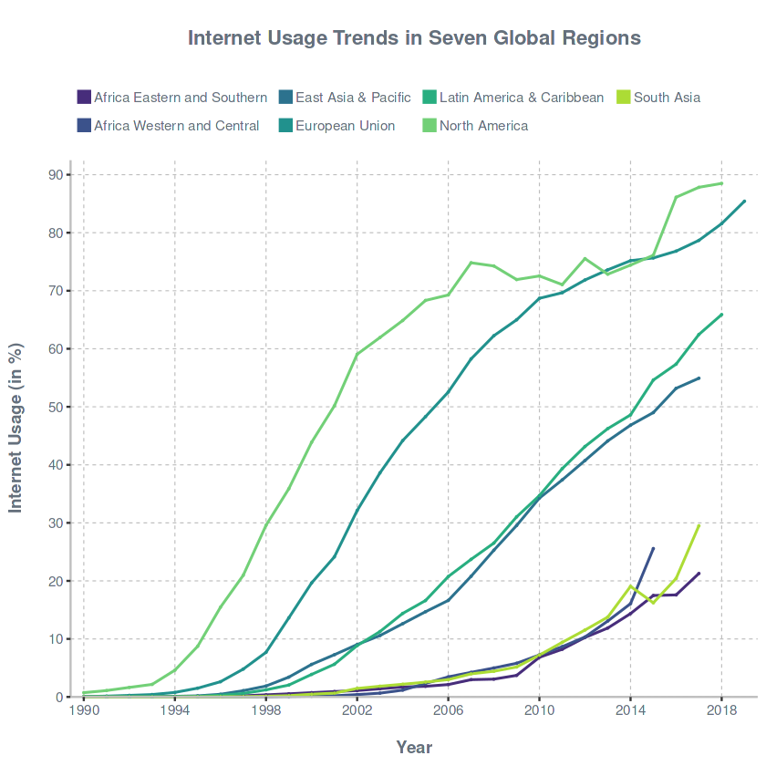
What are the top five (5) countries with the highest internet use for each of the following regions: Africa Eastern and Southern, Africa Western and Central, Latin America & Caribbean, East Asia & Pacific, South Asia, North America, and European Union? How do we describe these regions’ internet usage over time?
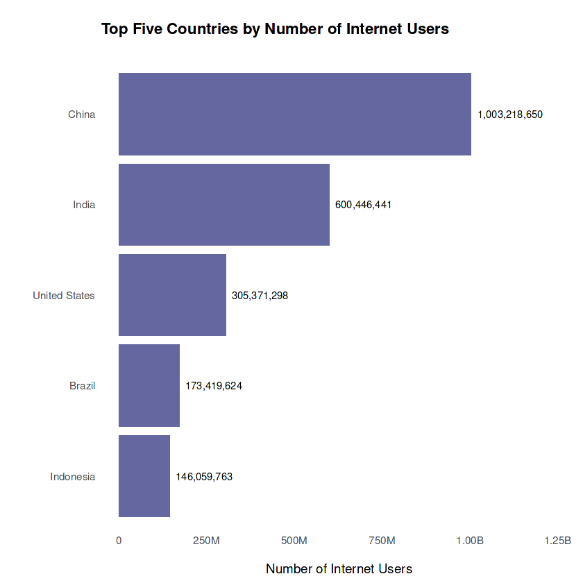
What are the top five (5) countries with the most internet users?
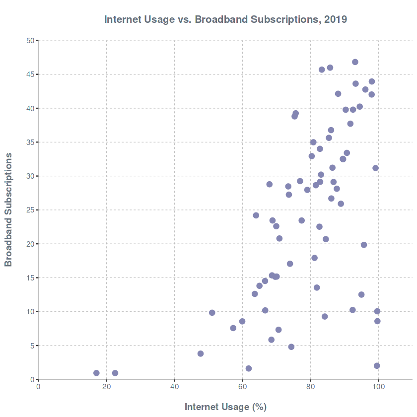
What is the correlation between internet usage (population share) and broadband subscriptions for 2019?

1.2. Libraries & Functions

# Load required packages
library(tidyverse)
library(dplyr)
library(ggplot2)
library(scales)
library(scales) # used for percentage values
library(countrycode) # identify the region of a country

# Create a function for plotting time series in ggplot
plot_series <- function(
    data = NULL,
    x = NULL,
    xlabs = "",
    y = NULL,
    ylabs = "",
    group = NULL,
    title = "",
    title.s = 10,
    by = 10,
    colors = NULL
) {
    
    # Plot
    p <- data %>%
        ggplot(aes(x = !!sym(x), 
                   y = !!sym(y),
                   group = !!sym(group))) + 
        	geom_line(aes(color = !!sym(group)),
                    	  linewidth = 0.65) +
        	geom_point(aes(color = !!sym(group)), 
                           size = 0) +
        	theme(legend.position = "top",
                  legend.justification = -0.12,
                  legend.direction = "horizontal",
                  legend.key.size = unit(0, 'pt'),
                  legend.text = element_text(margin = margin(r = 5, unit = "pt"),
                                             color = "#65707C"),
                  legend.title = element_blank(),
                  legend.key = element_blank(),
                  axis.title = element_text(color = "#65707C",
                                            face = "bold"),
                  axis.text = element_text(color = "#65707C"),
                  axis.line = element_line(colour = "grey",
                                           linewidth = 0.5),
                  panel.grid.major = element_line(color = "grey",
                                                  linetype = "dashed",
                                                  linewidth = 0.25),
                  panel.background = element_blank(),
                  plot.title = element_text(color = "#65707C",
                                            hjust = 0.5,
                                            size = title.s,
                                            face = "bold")
                 ) +
        	labs(x = paste0("\n",xlabs), y = paste0(ylabs,"\n")) +
        	ggtitle(paste0("\n",title,"\n")) +
        	scale_x_continuous(expand = c(0.02, 0),
    						   limits = c(min(data[x]), 2019), 
    						   breaks = seq(min(data[x]), 2019, by = 4)
            ) +
        	scale_y_continuous(expand = c(0, 0),
    						   limits = c(min(data[y]), max(data[y])+4), 
    						   breaks = seq(min(data[y]), max(data[y]+4), by = by)
            ) +
            guides(color = guide_legend(
                       override.aes = list(
                				 shape = 15,
                				 size = 4,
                                 linetype = "blank"
                       )
                   )
            )
    
    if (!is.null(colors)) {
        p <- p + scale_color_manual(values = colors)    
    }

    print(p)
}

# Create a function for plotting bar graphs in ggplot
plot_bar <- function(
    data = NULL,
    group = "",
    xlabs = "",
    num = "",
    ylabs = "",
    title = "",
    title.s = 10
) {
    ggplot(data, aes(y = fct_reorder(!!sym(group), !!sym(num)), x = !!sym(num))) + 
    geom_col(fill = "#6568A0") +
	#coord_flip() +
	geom_text(aes(label = comma_format()(!!sym(num)), y = !!sym(group), x = !!sym(num)),
              hjust = -0.1,
              size = 3.0
    ) +
	theme_minimal() +
	theme(panel.grid.major = element_blank(),
          panel.grid.minor = element_blank(),
          plot.title = element_text(face = "bold", size = title.s)
    ) +
    labs(x = paste0("\n",xlabs), y = paste0(ylabs,"\n")) +
    ggtitle(paste0("\n",title,"\n")) +
	scale_x_continuous(labels = scales::label_number(scale_cut = cut_short_scale()),
                       expand = expansion(mult = c(0.05, 0.30))
    )
}

1.3. Datasets

The following datasets are part of The World Bank’s World Development Indicators (WDI).

# Read data from CSV files
internet <- read_csv('data/internet.csv', show_col_types = FALSE)
people <- read_csv('data/people.csv', show_col_types = FALSE)
broadband <- read_csv('data/broadband.csv', show_col_types = FALSE)

1.3.1. Internet

Variable	Description
Entity	Name of the country, region, or group
Code	Unique id for the country (null for other entities)
Year	Year from 1990 to 2019
Internet_Usage	Share of the entity’s population who have used the internet in the last three months

# View the 'internet' dataset
head(internet)
tail(internet)

Entity	Code	Year
Afghanistan	AFG	1990
Afghanistan	AFG	1991
Afghanistan	AFG	1992
Afghanistan	AFG	1993
Afghanistan	AFG	1994
Afghanistan	AFG	1995

Entity	Code	Year	Internet_Usage
Zimbabwe	ZWE	2012	12.00000
Zimbabwe	ZWE	2013	15.50000
Zimbabwe	ZWE	2014	16.36474
Zimbabwe	ZWE	2015	22.74282
Zimbabwe	ZWE	2016	23.11999
Zimbabwe	ZWE	2017	27.05549

1.3.2. People

Variable	Description
Entity	Name of the country, region, or group
Code	Unique id for the country (null for other entities)
Year	Year from 1990 to 2020
Users	Number of people who have used the internet in the last three months for that country, region, or group

# View the 'people' dataset
head(people)
tail(people)

Entity	Code	Year
Afghanistan	AFG	1990
Afghanistan	AFG	1991
Afghanistan	AFG	1992
Afghanistan	AFG	1993
Afghanistan	AFG	1994
Afghanistan	AFG	1995

Entity	Code	Year	Users
Zimbabwe	ZWE	2015	3219232
Zimbabwe	ZWE	2016	3341464
Zimbabwe	ZWE	2017	3599269
Zimbabwe	ZWE	2018	3763048
Zimbabwe	ZWE	2019	3854006
Zimbabwe	ZWE	2020	4591211

1.3.3. Broadband

Variable	Description
Entity	Name of the country, region, or group
Code	Unique id for the country (null for other entities)
Year	Year from 1998 to 2020
Broadband_Subscriptions	Number of fixed subscriptions to high-speed internet at downstream speeds >= 256 kbit/s for that country, region, or group

# View the 'broadband' dataset
head(broadband)
tail(broadband)

Entity	Code	Year	Broadband_Subscriptions
Afghanistan	AFG	2004	0.000808843
Afghanistan	AFG	2005	0.000857557
Afghanistan	AFG	2006	0.001891571
Afghanistan	AFG	2007	0.001844982
Afghanistan	AFG	2008	0.001803604
Afghanistan	AFG	2009	0.003521770

Entity	Code	Year	Broadband_Subscriptions
Zimbabwe	ZWE	2015	1.187053
Zimbabwe	ZWE	2016	1.217633
Zimbabwe	ZWE	2017	1.315694
Zimbabwe	ZWE	2018	1.406322
Zimbabwe	ZWE	2019	1.395818
Zimbabwe	ZWE	2020	1.368916

2. Results and Discussion

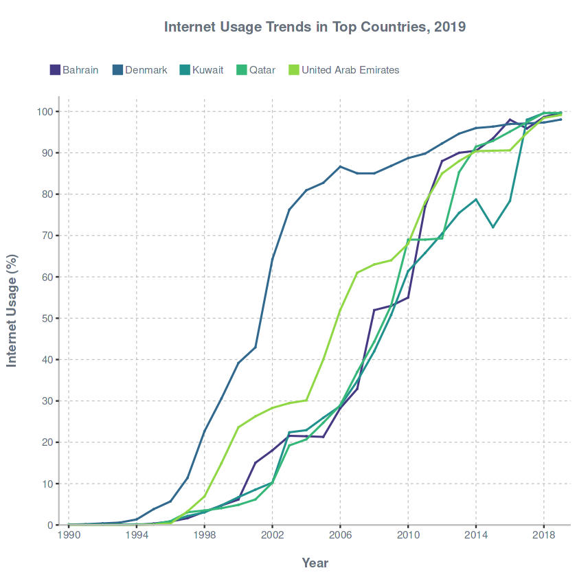
Based on the most recent 2019 data, four of the top five countries with the highest internet usage by population share are located in the Middle East. These countries are Bahrain, Qatar, Kuwait, and the United Arab Emirates (UAE).

# Top 5 countries with the highest internet use by population share
top_five_internet_use <- internet %>%
    group_by(Entity) %>% 
	filter(Year == 2019) %>%
    arrange(desc(Internet_Usage)) %>%
    ungroup() %>%
    top_n(5, Internet_Usage) %>%
	mutate(Internet_Usage = label_percent(accuracy = 0.01)(Internet_Usage/100)) %>%
	select(c("Entity", "Internet_Usage")) %>%
	rename(Country = Entity)

Country	Internet_Usage
Bahrain	99.70%
Qatar	99.65%
Kuwait	99.54%
United Arab Emirates	99.15%
Denmark	98.05%

# Top 5 countries with the highest internet use by population share
top_five_internet_use <- internet %>%
    group_by(Entity) %>% 
	filter(Year == 2019) %>%
    arrange(desc(Internet_Usage)) %>%
    ungroup() %>%
    top_n(5, Internet_Usage) %>%
	mutate(Internet_Usage = label_percent(accuracy = 0.01)(Internet_Usage/100)) %>%
	select(c("Entity", "Internet_Usage")) %>%
	rename(Country = Entity)

# Subset data for plot
plotData_top_five_internet_use <- internet %>% filter(Entity %in% top_five_internet_use$Country)

# Plot time series
plot_series(
    data = plotData_top_five_internet_use,
    x = "Year",
    xlabs = "Year",
    y = "Internet_Usage",
    ylabs = "Internet Usage (%)",
    group = "Entity",
    title = "Internet Usage Trends in Top Countries, 2019",
    title.s = 12,
    colors = c("#443A83", "#31688E", "#21918D", "#35B779", "#8FD744")
)

Internet Usage Trends in Top Countries, 2019

2.2. Top Countries’ Number of Internet Users, 2019

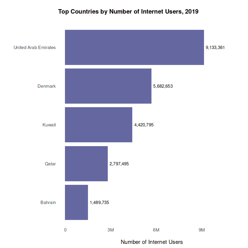
Among these countries, the United Arab Emirates (UAE) had the highest number of internet users in 2019.

# Number of internet users in 2019 of the countries with the highest internet use by population share
top_five_internet_users_2019 <- people %>% 
  filter(Entity %in% top_five_internet_use$Country, Year == 2019) %>%
  arrange(desc(Users)) %>% 
  mutate(Users = comma_format()(Users)) %>%
  select(c("Entity", "Users")) %>%
  rename(Country = Entity, Number_of_Internet_Users = Users)

# Subset data for plot
barData_top_five_internet_users_2019 <- people %>%
  filter(Entity %in% top_five_internet_users_2019$Country, Year == 2019) %>%
  arrange(desc(Users)) %>%
  select(c("Entity", "Users"))

# Plot bar graph
plot_bar(
    data = barData_top_five_internet_users_2019, #NULL,
    group = "Entity",
    xlabs = "Number of Internet Users",
    num = "Users",
    ylabs ="",
    title = "Top Countries by Number of Internet Users, 2019",
    title.s = 12
)

Top Countries by Number of Internet Users, 2019

2.3. Regional Leaders in Internet Usage

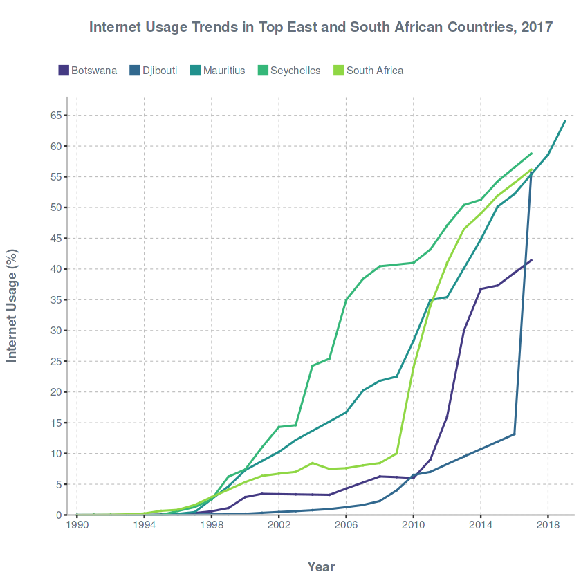
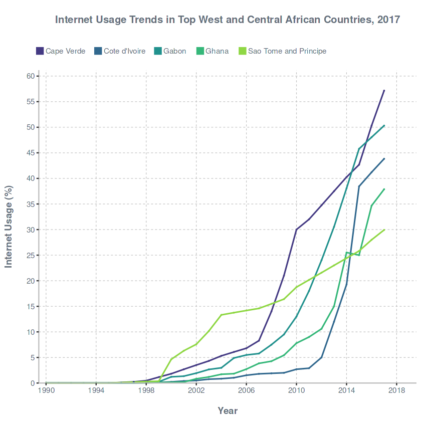
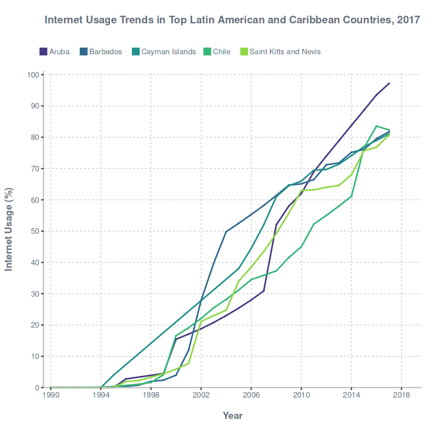
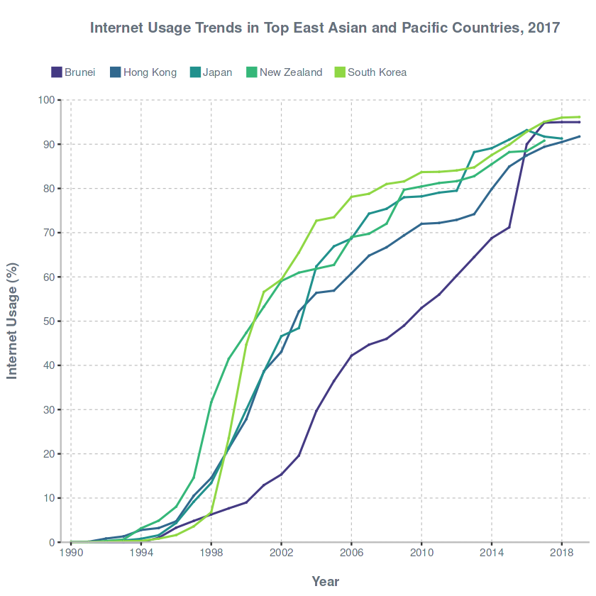
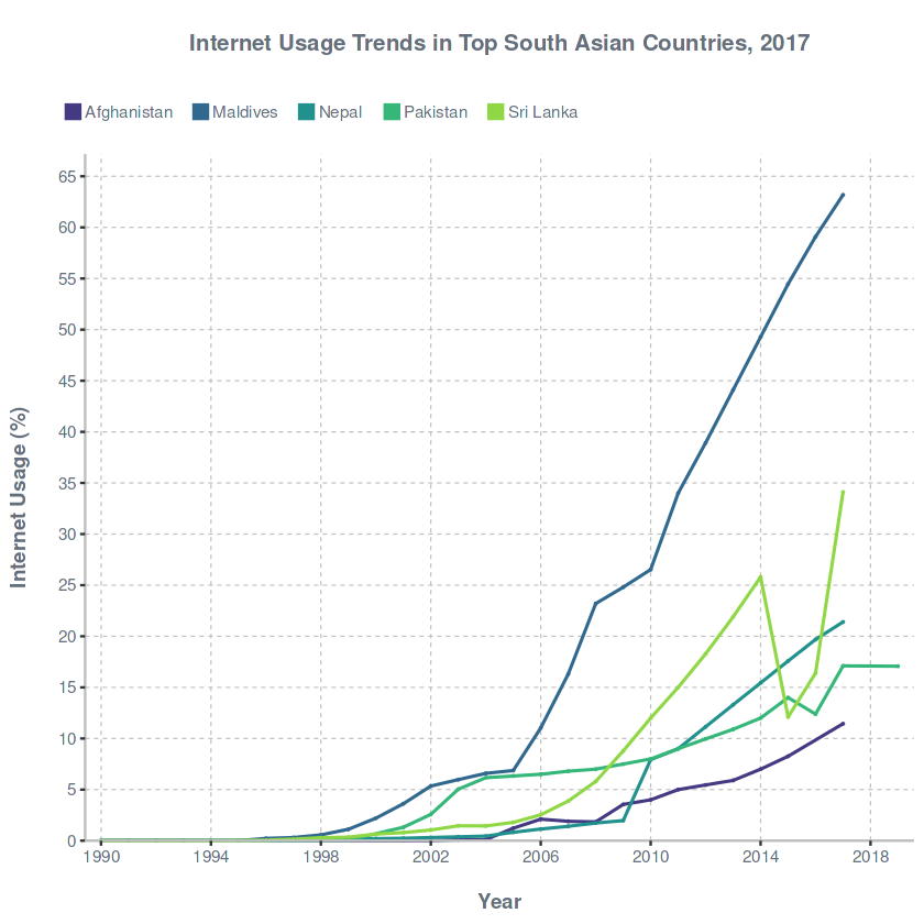
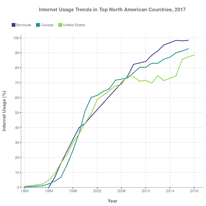
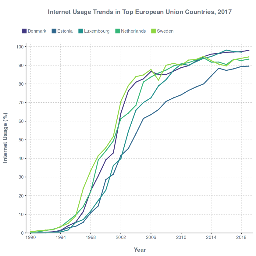
The countries with the highest internet usage by population share in their respective regions are Seychelles (Africa Eastern and Southern), Cape Verde (Africa Western and Central), Aruba (Latin America & Caribbean), South Korea (East Asia & Pacific), Maldives (South Asia), Bermuda (North America), and Luxembourg (European Union).
Notably, these countries are generally not the largest in terms of land area when compared to others.

Note: The 2017 data was used for this comparison because it was the most recent year with the most available country data.

# The 'region' destination (7 Regions as defined in the World Bank Development Indicators) was used for Latin America & Caribbean, East Asia & Pacific, South Asia, and North America.
code_region <- distinct(data.frame( Code = (internet %>% filter(Code != 'null'))$Code, 
               		Region = countrycode((internet %>% filter(Code != 'null'))$Code, 
                  		'wb', 'region')), Code, .keep_all = TRUE) %>% 
				  		filter(Code != 'OWID_WRL') %>%
			     		mutate(Region = ifelse(Code == 'OWID_KOS', 'Europe & Central Asia', Region)) 

# The 'region23' destination (23 Regions as used to be in the World Bank Development Indicators) was used for Africa Eastern and Southern and Africa Western and Central.
code_region23 <- distinct(data.frame(Code = (internet %>% filter(Code != 'null'))$Code, 
                 	Region = countrycode((internet %>% filter(Code != 'null'))$Code, 
                  		'wb', 'region23')), Code, .keep_all = TRUE) %>%
				  		filter(Code != 'OWID_WRL') %>%
			     		mutate(Region = ifelse(Code == 'OWID_KOS', 'Southern Europe', Region)) 

# Join 'Code' from 'internet' to 'code_region' and 'code_region23' tables to identify a country's region
internet_with_region <- merge(internet, code_region, by = 'Code', all = TRUE)
internet_with_region23 <- merge(internet, code_region23, by = 'Code', all = TRUE)

# The country Kosovo was not matched**, so its regions(https://data.worldbank.org/country/XK) was inputted manually. 
# The row with a Code = 'OWID_WRL' for World was excluded in the analysis.
# Since EU codes are incompatible, a different coding approach was used.

2.3.1. Africa Eastern and Southern

# Top five countries
top_five_internet_use_aes <- internet_with_region23 %>%
    group_by(Entity) %>% 
  filter(Year == 2017, Region %in% c('Eastern Africa', 'Southern Africa')) %>%
    arrange(desc(Internet_Usage)) %>%
    ungroup() %>%
    top_n(5, Internet_Usage) %>%
  mutate(Internet_Usage = label_percent(accuracy = 0.01)(Internet_Usage/100)) %>%
  select(c("Entity", "Internet_Usage")) %>%
  rename(Country = Entity)

Country	Internet_Usage
Seychelles	58.77%
South Africa	56.17%
Djibouti	55.68%
Mauritius	55.40%
Botswana	41.41%

# Subset data for plot
plotData_top_five_aes <- internet %>% filter(Entity %in% top_five_internet_use_aes$Country) 

# Plot time series
plot_series(
    data = plotData_top_five_aes,
    x = "Year",
    xlabs = "\nYear",
    y = "Internet_Usage",
    ylabs = "Internet Usage (%)\n",
    group = "Entity",
    title = "Internet Usage Trends in Top East and South African Countries, 2017",
    title.s = 12,
    by = 5,
    colors = c("#443A83", "#31688E", "#21918D", "#35B779", "#8FD744")
)

Internet Usage Trends in Top East and South African Countries, 2017

2.3.2. Africa Western and Central

# Top five countries
top_five_internet_use_awc <- internet_with_region23 %>%
    group_by(Entity) %>% 
  filter(Year == 2017, Region %in% c('Western Africa', 'Middle Africa')) %>%
    arrange(desc(Internet_Usage)) %>%
    ungroup() %>%
    top_n(5, Internet_Usage) %>%
  mutate(Internet_Usage = label_percent(accuracy = 0.01)(Internet_Usage/100)) %>%
  select(c("Entity", "Internet_Usage")) %>%
  rename(Country = Entity)

Country	Internet_Usage
Cape Verde	57.16%
Gabon	50.32%
Cote d'Ivoire	43.84%
Ghana	37.88%
Sao Tome and Principe	29.93%

# Subset data for plot
plotData_top_five_awc <- internet %>% filter(Entity %in% top_five_internet_use_awc$Country) 

# Plot time series
plot_series(
    data = plotData_top_five_awc,
    x = "Year",
    xlabs = "Year",
    y = "Internet_Usage",
    ylabs = "Internet Usage (%)",
    group = "Entity",
    title = "Internet Usage Trends in Top West and Central African Countries, 2017",
    title.s = 12,
    by = 5,
    colors = c("#443A83", "#31688E", "#21918D", "#35B779", "#8FD744")
)

Internet Usage Trends in Top West and Central African Countries, 2017

2.3.3. Latin America & Caribbean

# Top five countries
top_five_internet_use_lac <- internet_with_region %>%
    distinct(Internet_Usage, .keep_all = TRUE) %>%
    group_by(Entity) %>% 
	filter(Year == 2017, Region == 'Latin America & Caribbean') %>%
    arrange(desc(Internet_Usage)) %>%
    ungroup() %>%
    top_n(5, Internet_Usage) %>%
	mutate(Internet_Usage = label_percent(accuracy = 0.01)(Internet_Usage/100)) %>%
	select(c("Entity", "Internet_Usage")) %>%
	rename(Country = Entity)

Country	Internet_Usage
Aruba	97.17%
Chile	82.33%
Barbados	81.76%
Cayman Islands	81.07%
Saint Kitts and Nevis	80.71%

# Subset data for plot
plotData_top_five_lac <- internet %>% filter(Entity %in% top_five_internet_use_lac$Country) 

# Plot time series
plot_series(
    data = plotData_top_five_lac,
    x = "Year",
    xlabs = "Year",
    y = "Internet_Usage",
    ylabs = "Internet Usage (%)",
    group = "Entity",
    title = "Internet Usage Trends in Top Latin American and Caribbean Countries, 2017",
    title.s = 12,
    by = 10,
    colors = c("#443A83", "#31688E", "#21918D", "#35B779", "#8FD744")
)

Internet Usage Trends in Top Latin American and Caribbean Countries, 2017

2.3.4. East Asia & Pacific

# Top five countries
top_five_internet_use_eap <- internet_with_region %>%
    distinct(Internet_Usage, .keep_all = TRUE) %>%
    group_by(Entity) %>% 
  filter(Year == 2017, Region == 'East Asia & Pacific') %>%
    arrange(desc(Internet_Usage)) %>%
    ungroup() %>%
    top_n(5, Internet_Usage) %>%
  mutate(Internet_Usage = label_percent(accuracy = 0.01)(Internet_Usage/100)) %>%
  select(c("Entity", "Internet_Usage")) %>%
  rename(Country = Entity)

Country	Internet_Usage
South Korea	95.07%
Brunei	94.87%
Japan	91.73%
New Zealand	90.81%
Hong Kong	89.42%

# Subset data for plot
plotData_top_five_eap <- internet %>% filter(Entity %in% top_five_internet_use_eap$Country) 

# Plot time series
plot_series(
    data = plotData_top_five_eap,
    x = "Year",
    xlabs = "Year",
    y = "Internet_Usage",
    ylabs = "Internet Usage (%)",
    group = "Entity",
    title = "Internet Usage Trends in Top East Asian and Pacific Countries, 2017",
    title.s = 12,
    by = 10,
    colors = c("#443A83", "#31688E", "#21918D", "#35B779", "#8FD744")
)

Internet Usage Trends in Top East Asian and Pacific Countries, 2017

2.3.5. South Asia

# Top five countries
top_five_internet_use_sa <- internet_with_region %>%
    distinct(Internet_Usage, .keep_all = TRUE) %>%
    group_by(Entity) %>% 
  filter(Year == 2017, Region == 'South Asia') %>%
    arrange(desc(Internet_Usage)) %>%
    ungroup() %>%
    top_n(5, Internet_Usage) %>%
  mutate(Internet_Usage = label_percent(accuracy = 0.01)(Internet_Usage/100)) %>%
  select(c("Entity", "Internet_Usage")) %>%
  rename(Country = Entity)

Country	Internet_Usage
Maldives	63.19%
Sri Lanka	34.11%
Nepal	21.40%
Pakistan	17.11%
Afghanistan	11.45%

# Subset data for plot
plotData_top_five_sa <- internet %>% filter(Entity %in% top_five_internet_use_sa$Country) 

# Plot time series
plot_series(
    data = plotData_top_five_sa,
    x = "Year",
    xlabs = "Year",
    y = "Internet_Usage",
    ylabs = "Internet Usage (%)",
    group = "Entity",
    title = "Internet Usage Trends in Top South Asian Countries, 2017",
    title.s = 12,
    by = 5,
    colors = c("#443A83", "#31688E", "#21918D", "#35B779", "#8FD744")
)

Internet Usage Trends in Top South Asian Countries, 2017

2.3.6. North America

# Top countries
top_internet_use_na <- internet_with_region %>%
    distinct(Internet_Usage, .keep_all = TRUE) %>%
    group_by(Entity) %>% 
  filter(Year == 2017, Region == 'North America') %>%
    arrange(desc(Internet_Usage)) %>%
    ungroup() %>%
    top_n(5, Internet_Usage) %>%
  mutate(Internet_Usage = label_percent(accuracy = 0.01)(Internet_Usage/100)) %>%
  select(c("Entity", "Internet_Usage")) %>%
  rename(Country = Entity)

Country	Internet_Usage
Bermuda	98.37%
Canada	92.70%
United States	87.27%

# Subset data for plot
plotData_top_na <- internet %>% filter(Entity %in% top_internet_use_na$Country) 

# Plot time series
plot_series(
    data = plotData_top_na,
    x = "Year",
    xlabs = "Year",
    y = "Internet_Usage",
    ylabs = "Internet Usage (%)",
    group = "Entity",
    title = "Internet Usage Trends in Top North American Countries, 2017",
    title.s = 12,
    by = 10,
    colors = c("#443A83", "#21918D", "#8FD744")
)

Internet Usage Trends in Top North American Countries, 2017

2.3.7. European Union

# EU country codes
EUCodes <- data.frame(
  Code = c('AUT', 'BEL', 'BGR', 'HRV', 'CYP', 'CZE', 'DNK', 'EST', 'FIN', 'FRA', 'DEU', 'GRC', 'HUN',	'IRL', 'ITA', 'LVA', 'LTU', 'LUX', 'MLT', 'NLD', 'POL', 'PRT', 'ROU', 'SVK', 'SVN', 'ESP', 'SWE'),
  Region = replicate(27, 'European Union')
)

# https://www23.statcan.gc.ca/imdb/p3VD.pl?Function=getVD&TVD=141329
# This list was used for the country codes. As of writing, there are only twenty-seven (27) members (https://european-union.europa.eu/principles-countries-history/country-profiles_en), which means that United Kingdom was excluded from after formally leaving in 2020 (https://www.ema.europa.eu/en/about-us/history-ema/brexit-united-kingdoms-withdrawal-european-union).

# Join 'Code' from the internet and EUCodes tables to identify a country's region 
internet_eu <- merge(internet, EUCodes, by = 'Code', all = TRUE) %>%
  filter(Region == 'European Union')

# Top five countries
top_five_internet_use_eu <- internet_eu %>%
    distinct(Internet_Usage, .keep_all = TRUE) %>%
    group_by(Entity) %>% 
  filter(Year == 2017, Region == 'European Union') %>%
    arrange(desc(Internet_Usage)) %>%
    ungroup() %>%
    top_n(5, Internet_Usage) %>%
  mutate(Internet_Usage = label_percent(accuracy = 0.01)(Internet_Usage/100)) %>%
  select(c("Entity", "Internet_Usage")) %>%
  rename(Country = Entity)

Country	Internet_Usage
Luxembourg	97.36%
Denmark	97.10%
Netherlands	93.20%
Sweden	93.01%
Estonia	88.10%

# Subset data for plot
plotData_top_five_eu <- internet %>% filter(Entity %in% top_five_internet_use_eu$Country) 

# Plot time series
plot_series(
    data = plotData_top_five_eu,
    x = "Year",
    xlabs = "Year",
    y = "Internet_Usage",
    ylabs = "Internet Usage (%)",
    group = "Entity",
    title = "Internet Usage Trends in Top European Union Countries, 2017",
    title.s = 12,
    by = 10,
    colors = c("#443A83", "#31688E", "#21918D", "#35B779", "#8FD744")
)

Internet Usage Trends in Top European Union Countries, 2017

2.4. Internet Usage by Region

# Top five countries per region
highlights <- rbind(
    top_five_internet_use_aes %>% mutate(Region="Africa Eastern and Southern"),
    top_five_internet_use_awc %>% mutate(Region="Africa Western and Central"),
    top_five_internet_use_lac %>% mutate(Region="Latin America & Caribbean"),
    top_five_internet_use_eap %>% mutate(Region="East Asia & Pacific"), 
    top_five_internet_use_sa %>% mutate(Region="South Asia"),
    top_three_internet_use_na %>% mutate(Region="North America"),
    top_five_internet_use_eu %>% mutate(Region="European Union")
)

# Top country per region
top_countries <- highlights %>%
    group_by(Region) %>%
    top_n(1, Internet_Usage)

# Internet usages of regions of interest
internet_regionsOfInterest <- rbind(
    internet_with_region %>% 
      filter(Region %in% c('Latin America & Caribbean', 
                             'East Asia & Pacific', 
                             'South Asia', 
                             'North America')),
    internet_with_region23 %>% 
      filter(Region %in% c('Eastern Africa', 
                             'Southern Africa', 
                             'Western Africa',  
                             'Middle Africa')) %>%
        mutate(Region = ifelse(Region %in% c('Eastern Africa','Southern Africa'),
                                'Africa Eastern and Southern', 'Africa Western and Central')),
    internet_eu
)

# Most recent data for the 'Africa Western and Central' region
most_recent_awc <- internet %>%
  filter(Year == 2015, Entity == 'Africa Western and Central')

# Seven regions' internet usages in 2017
internetUsage_regions <- internet %>%
  filter(Year == 2017, Entity %in% internet_regionsOfInterest$Region) %>%
  bind_rows(most_recent_awc) %>%
  mutate(Internet_Usage = label_percent(accuracy = 0.01)(Internet_Usage/100)) %>%
  select(c("Entity", "Internet_Usage")) %>%
  rename (Region = Entity) %>%
  arrange(desc(Internet_Usage))

Region	Internet_Usage
North America	87.83%
European Union	78.68%
Latin America & Caribbean	62.47%
East Asia & Pacific	54.93%
South Asia	29.50%
Africa Western and Central	25.57%
Africa Eastern and Southern	21.28%

# Subset data for plot
plotData_region_internet <- internet %>% filter(Entity %in% internet_regionsOfInterest$Region)

# Plot time series
plot_series(
    data = plotData_region_internet,
    x = "Year",
    xlabs = "Year",
    y = "Internet_Usage",
    ylabs = "Internet Usage (in %)",
    group = "Entity",
    title = "Internet Usage Trends in Seven Global Regions",
    title.s = 13,
    by = 10,
    colors = c("#472D7B", "#3B528B", "#2C728E", "#21918D", "#28AE80", "#72D077", "#ACDC35")
)

Internet Usage Trends in Seven Global Regions

2.5. Countries with the Most Internet Users

Based on the World Population Review, all of these countries are among the top ten most populous nations, with four of them also ranking in the top five (excluding Brazil).

# Top five countries
top_five_internet_users <- people %>%
    group_by(Entity) %>% 
  filter(Year == max(Year), Code != 'null', Entity != 'World') %>%
    arrange(desc(Users)) %>%
    ungroup() %>%
    top_n(5, Users) %>%
  select(c("Entity", "Users"))

# Plot bar graph
plot_bar(
    data = top_five_internet_users,
    group = "Entity",
    xlabs = "Number of Internet Users",
    num = "Users",
    ylabs = "",
    title = "Top Five Countries by Number of Internet Users",
    title.s = 13
)

Top Five Countries by Number of Internet Users

2.6. Relationship Between Internet Usage & Broadband Subscriptions, 2019

The correlational analysis revealed a moderately high positive correlation (\(r = 0.56\)) between internet usage and broadband subscriptions in 2019, which is statistically significant at a 0.01 level (\(p = 4.914e^{-07}\)), allowing us to reject the null hypothesis of no correlation.
We are at least 99% confident that the true correlation coefficient (\(ρ\)) lies within the range of 0.3730 to 0.7018.
This positive relationship is also visually apparent in the scatter plot below.

# Join 'internet' and 'broadband' tables
internet_and_broadband_2019 <- internet %>% 
  inner_join(broadband, by = c("Entity", "Code", "Year")) %>%
    filter(Year == 2019)

# Perform a Pearson correlation test
pearson_corr <- data.frame(
  Correlation_Coefficient = cor.test(internet_and_broadband_2019$Internet_Usage,
                        internet_and_broadband_2019$Broadband_Subscriptions,
                        method = "pearson")$estimate,
  P=cor.test(internet_and_broadband_2019$Internet_Usage,
                     internet_and_broadband_2019$Broadband_Subscriptions,
                     method = "pearson")$p.value,
  CI_Lower=(cor.test(internet_and_broadband_2019$Internet_Usage,
                       internet_and_broadband_2019$Broadband_Subscriptions,
                       method = "pearson")$conf.int)[1],
  CI_Upper=(cor.test(internet_and_broadband_2019$Internet_Usage,
                       internet_and_broadband_2019$Broadband_Subscriptions,
                       method = "pearson")$conf.int)[2]	
)
rownames(pearson_corr) <- "Value"

	Correlation_Coefficient	P	CI_Lower	CI_Upper
Value	0.5590077	4.913904e-07	0.3730323	0.7017988

# Plot scatter points
scatter_for_corr <- ggplot(internet_and_broadband_2019, aes(x = Internet_Usage, y = Broadband_Subscriptions)) +
  geom_point(color = "#8486B3", size = 2.5) +
    theme(legend.position = "top",
        legend.justification = -0.12,
        legend.direction = "horizontal",
        legend.key.size = unit(0, 'pt'),
        legend.text = element_text(margin = margin(r = 5, unit = "pt"), color = "#65707C"),
        legend.title = element_blank(),
        legend.key = element_blank(),
        axis.title = element_text(color = "#65707C", face = "bold"),
        axis.text = element_text(color = "#65707C"),
        axis.line = element_line(colour = "grey", linewidth = 0.5),
        panel.grid.major = element_line(color = "grey", linetype = "dashed", linewidth = 0.25),
        panel.background = element_blank(),
        plot.title = element_text(color = "#65707C",
                                  hjust = 0.5,
                                  size = 12,
                                  face = "bold")
        ) +
  labs(x = '\nInternet Usage (%)', y = 'Broadband Subscriptions\n') +
  ggtitle("\nInternet Usage vs. Broadband Subscriptions, 2019\n") +
  scale_x_continuous(expand = c(0.00, 0),
                       limits = c(0, 110), 
                       breaks = seq(0, 100, by = 20)) +
  scale_y_continuous(expand = c(0.00, 0),
                       limits = c(0, 50),
                       breaks = seq(0, 50, by = 5))

Internet Usage vs. Broadband Subscriptions, 2019

3. Conclusion

Based on the data and results of the analyses, the following conclusions can be drawn about the global state of internet accessibility:

The highest internet usage by population share worldwide is concentrated in several Middle Eastern countries.
Western regions experienced a significantly quicker growth in internet accessibility compared to their eastern counterparts.
The countries with the highest internet usage within a region are not necessarily those with the largest land areas.
Conversely, the most populous countries tend to have the greatest total number of internet users.
In 2019, countries with a higher percentage of internet users in their population also had a corresponding increase in fixed broadband subscriptions (at downstream speeds of 256 kbit/s or more).

Share on

Bluesky Facebook LinkedIn X (formerly Twitter)

Jon Bon Jovi Dela Cruz